
Make fgmax_grid data for Copalis Beach#
This Jupyter notebook is available in $GTT/CopalisBeach/example3/make_fgmax_grid_Copalis.ipynb within the
GeoClaw Tsunami Tutorial.
Creates an fgmax grid for point_style==4 in GeoClaw covering the points around Copalis Beach that are below some specified elevation. Instead of specifying a regular 2D grid and monitoring fgmax values at every point on the grid (as was done in Copalis Beach example2), a file is created in the format of a topofile that has 0/1 values at each grid point indicating whether fgmax values should be monitored at that point or not.
For this example we start with a desired fgmax region that extends farther north than the fgmax grid used in Copalis Beach example2, so that it contains many points in the hills north of town that are so high we know in advance that the tsunami will not reach them, and hence it would be a waste of effort to monitor them.
For this example we go down to 1/3 arcsecond resolution on the finest grid and specify the fgmax points by starting with the topo file $GTT/topo/topofiles/Copalis_13s.asc at this resolution, cropped to the desired fgmax_extent = [-124.2, -124.155, 47.11, 47.18]. The cropped DEM is 756 x 486 and contains 367416 points. By selecting only the points that have elevation less than 30 m (relative to MHW), we can reduce this to only 284092 fgmax points. These numbers are calculated below.
Note that what elevation we should choose as our cutoff will depend on the event(s) we plan to model and the nature of the topography. Large near-field events will typically inundate to higher elevations than small events or far-field tsunamis. Steep canyons near the coast may focus waves and can experience inundation to much greater elevations than would be seen on a gentle coastal plane. Some experimentation may be needed in practice.
The results shown in the fgmax_results notebook indicate that for the problem being solved here, the elevation of 30m is not sufficient if one is interested in capturing the highest inundation values in some narrow canyons to the north of Copalis Beach, or on the high bluffs along the river. However, if the goal is to model inunduation only in regions around the town, then this is sufficient and in fact a smaller cutoff value (and perhaps smaller fgmax region) would be sufficient.
See also
MarchingFront.ipynb in the Clawpack Gallery of Jupyter notebooks, has more details on the steps used in this notebook.
%matplotlib inline
from pylab import *
import os,sys
from clawpack.visclaw import colormaps, plottools
from clawpack.geoclaw import topotools, marching_front, kmltools, fgmax_tools
from clawpack.amrclaw import region_tools
from numpy import ma
import glob
import zipfile
Define some plotting functions and colormaps#
zmin = -70.
zmax = 35.
sea_level = 0.  # corresponding to MHW in coastal DEMs

cmap_land = colormaps.make_colormap({ 0.0:[0.1,0.4,0.0],
                                     0.25:[0.0,1.0,0.0],
                                      0.5:[0.8,1.0,0.5],
                                      1.0:[0.8,0.5,0.2]})

cmap_water = colormaps.make_colormap({ 0.0:[0,0,1], 1.:[.8,.8,1]})

cmap_topo, norm_topo = colormaps.add_colormaps((cmap_land, cmap_water),
                                     data_limits=(zmin,zmax),
                                     data_break=sea_level)


def plottopo(topo):
    figure(figsize=(13,8))
    plottools.pcolorcells(topo.X, topo.Y, topo.Z, cmap=cmap_topo, norm=norm_topo)
    colorbar(extend='both',shrink=0.5)
    gca().set_aspect(1./cos(47*pi/180.))
    xticks(rotation=20);

def plottopo_fgmax(selected=None):
    figure(figsize=(13,8))
    if selected is not None:
        Z = ma.masked_where(logical_not(selected), topo_fgmax.Z)
    else:
        Z = topo_fgmax.Z
    plottools.pcolorcells(topo_fgmax.X, topo_fgmax.Y, Z, cmap=cmap_topo, norm=norm_topo)
    colorbar(extend='both',shrink=0.5)
    gca().set_aspect(1./cos(47*pi/180.))
    xticks(rotation=20);
    ticklabel_format(useOffset=False)
Load topofile and crop to the desired fgmax extent#
topo = topotools.Topography('../../topo/topofiles/Copalis_13s.asc', 3)
*** Note: since grid registration is llcorner,
    will shift x,y values by (dx/2, dy/2) to cell centers
loc = 'CopalisBeach'
fgmax_extent = [-124.2, -124.155, 47.11, 47.18] # approximate desired extent
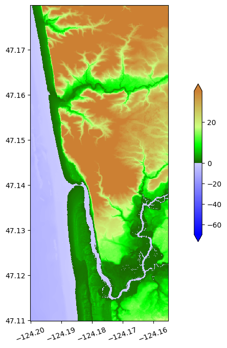
topo_fgmax = topo.crop(fgmax_extent)
print(f'The cropped region has shape {topo_fgmax.X.shape} and contains {prod(topo_fgmax.X.shape)} points')
The cropped region has shape (756, 486) and contains 367416 points
plottopo_fgmax()
Determine best computational domain edges#
Ideally, we would like the fgmax points to be centered within computational grid cells at the finest level (the level from which we plan to update the fgmax values during inundation). With fgmax point_style == 4, the fgmax point locations are determined by the existing topofile, so we may have to adjust the domain boundaries a bit so that these points are in computational cell centers.
For this example we assume that the finest level has cell width dx = 1/3 arcsecond, to agree with the resolution of the topofile that we are using. So in choosing our domain edge, we want to make sure that the fgmax points (= topo points) are all some distance (N + 0.5) * dx away from this edge, for some integer N.
In longitude, we want the left domain edge to be near -128.5, but we see that this will not work:
x_edge_desired = -128.5
dx = 1/(3*3600)
cellwidths = (topo_fgmax.x[0] - x_edge_desired)/dx
print(f'topo_fgmax.x[0] is {cellwidths:.4f} 1/3" cell widths from x_edge_desired = {x_edge_desired}')
topo_fgmax.x[0] is 46440.1666 1/3" cell widths from x_edge_desired = -128.5
But if we shift this by 1/9”, it does work:
x_edge = x_edge_desired - 1/(9*3600)
cellwidths = (topo_fgmax.x[0] - x_edge)/dx
print(f'topo_fgmax.x[0] is {cellwidths:.4f} 1/3" cell widths from x_edge = {x_edge}')
topo_fgmax.x[0] is 46440.4999 1/3" cell widths from x_edge = -128.50003086419753
Similarly, we want the lower edge in latitude to be approximately 45, but we must also shift this by 1/9” to achieve the desired alignment, with topo_fgmax.y[0] - y_edge being of the form (N + 0.5)*dy:
y_edge_desired = 45.
dy = 1/(3*3600)
cellwidths = (topo_fgmax.y[0] - y_edge_desired)/dy
print(f'topo_fgmax.y[0] is {cellwidths:.4f} 1/3" cell widths from y_edge_desired = {y_edge_desired}')

y_edge = y_edge_desired - 1/(9*3600)
cellwidths = (topo_fgmax.y[0] - y_edge)/dy
print(f'topo_fgmax.y[0] is {cellwidths:.4f} 1/3" cell widths from y_edge = {y_edge}')
topo_fgmax.y[0] is 22788.1666 1/3" cell widths from y_edge_desired = 45.0
topo_fgmax.y[0] is 22788.5000 1/3" cell widths from y_edge = 44.999969135802466
Modification to setrun#
So in our setrun.py file we should shift the domain edges by 1/9” and use
# Lower and upper edge of computational domain:
one_ninth_sec = 1 / (9*3600)

clawdata.lower[0] = -128.5 - one_ninth_sec     # west longitude
clawdata.upper[0] = -123.5 - one_ninth_sec     # east longitude

clawdata.lower[1] = 45. - one_ninth_sec        # south latitude
clawdata.upper[1] = 49. - one_ninth_sec        # north latitude

# Number of grid cells: Coarsest grid is 4 arcminutes (1/15 degree)
clawdata.num_cells[0] =  5*15
clawdata.num_cells[1] =  4*15
Note that we shift both the lower and upper edges in the same direction so that the distance clawdata.upper[j] - clawdata.lower[j] is still an integer number of degrees in each case, and so that the coarsest grid is still 4 arcminutes (and hence the finest grid level is still exactly 1/3 arcsecond), and all fgmax points are aligned with cell centers on this grid.
Select fgmax points below some elevation#
The reason for using point_style == 4 and specifying a topofile-like array is so that we only have to update fgmax points in regions where there is likely to be inundation, avoiding additional work in regions with high elevation.
So we choose fgmax points to include all those with an elevation less than some value Zmax, provided that these points can be reached from the ocean by a path of grid cells that is always less than this elevation. (This avoids choosing fgmax points in some low region that is isolated from the ocean by higher topography and hence protected from the tsunami.)
This selection is done by the marching front algorithm described in Marching Front Algorithm documentation.
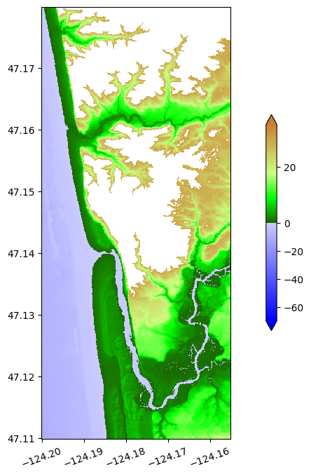
Zmax = 30.   # only select points below this elevation
fgmax_pts_chosen = marching_front.select_by_flooding(topo_fgmax.Z,
                                   Z1=0, Z2=Zmax, max_iters=None)
Selecting points with Z1 = 0, Z2 = 30, max_iters=367416
Done after 466 iterations with 271650 points chosen
plottopo_fgmax(fgmax_pts_chosen)
Remove offshore points, if desired#
Note that all offshore points are included in the fgmax_pts_chosen so far. If we were only interested in onshore inundation, we might want to only select onshore points (and perhaps nearshore points where the topography B is greater than some specified negative value, in particular to also capture the river in this example).
We do not do this here, see the example in the Marching Front Algorithm notebook from the GeoClaw documention if this is desired.
Add a few buffer points#
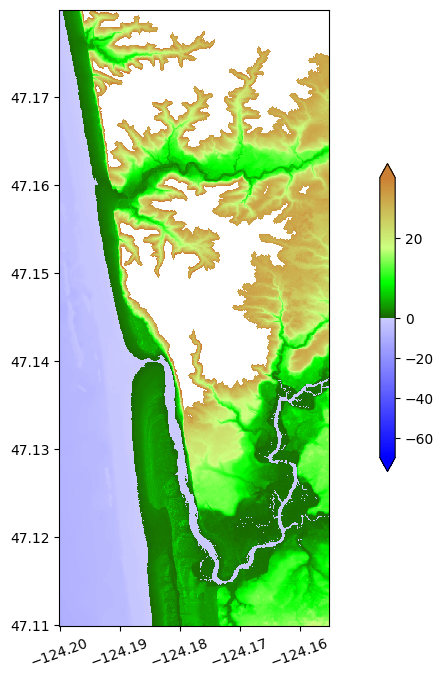
Note that along the river there are some high bluffs and so there is a sharp transition from low elevation to white areas in the plot above where fgmax is not monitored. It’s often safest to add a buffer region around the points selected so far, by taking a few iterations of the select_by_flooding algorithm with a very large value of Z2. Here we take max_iters = 2 iterations to expand the previously chosen points:
fgmax_pts_chosen = marching_front.select_by_flooding(topo_fgmax.Z,
                                Z1=0, Z2=1e6, prev_pts_chosen=fgmax_pts_chosen,
                                max_iters=2)
Selecting points with Z1 = 0, Z2 = 1e+06, max_iters=2
Done after 2 iterations with 284092 points chosen
plottopo_fgmax(fgmax_pts_chosen)
Check how many fgmax points we selected:#
Z_fgmax = ma.masked_array(topo_fgmax.Z, logical_not(fgmax_pts_chosen))
num_masked = Z_fgmax.mask.sum()
num_pts = prod(topo_fgmax.Z.shape)
print(f'Out of {num_pts} points in topo_fgmax.Z, {num_masked} are masked')
print(f'Number of fgmax points remaining is {num_pts - num_masked}')
Out of 367416 points in topo_fgmax.Z, 83324 are masked
Number of fgmax points remaining is 284092
Create the data file#
We now create a file fgmax_pts_CopalisBeach.data that will be used in the GeoClaw run to indicate what points should be used as fgmax points. This file has the form of a topofile with topo_type == 3 but rather than topography elevations in Z, it contains integers 1 or 0 to indicate whether each point on the uniform grid specified by the header is an fgmax point or not.
fgmax_pts_chosen = where(fgmax_pts_chosen, 1, 0)  # change boolean to 1/0
topo_fgmax_pts = topotools.Topography()
topo_fgmax_pts.set_xyZ(topo_fgmax.x, topo_fgmax.y, fgmax_pts_chosen)
fname_fgmax_pts = 'fgmax_pts_%s.data' % loc
topo_fgmax_pts.write(fname_fgmax_pts, topo_type=3, Z_format='%1i')
print('Created %s' % fname_fgmax_pts)
Created fgmax_pts_CopalisBeach.data
Make kml figures and files#
The remainder of this notebook creates a file fgmax_topo_CopalisBeach.kmz that can be opened in Google Earth to view the topography at the chosen fgmax points.
You can comment out the lines
close(fig)
to see what the figures look like that are incorporated in the kmz file, but note that they are large and lack axes for the purpose used here.
kml_dir = 'fgmax_kmlfiles_%s' % loc
os.system('mkdir -p %s' % kml_dir)
print('Will put png and kml files in %s' % kml_dir)
Will put png and kml files in fgmax_kmlfiles_CopalisBeach
# Make kml files showing extent of topo_fgmax:
kml_extent_dir = os.path.join(kml_dir, 'extents')
os.system('mkdir -p %s' % kml_extent_dir)
print('Will put extent kml files in %s' % kml_extent_dir)

name = loc + ' extent of topo_fgmax'
fname_topo_fgmax = '%s/topo_fgmax_extent.kml' % kml_extent_dir
kmltools.box2kml(topo_fgmax.extent, fname_topo_fgmax, name,
                 color='00FF00',width=1,verbose=True)

RR_extent = None
if RR_extent:
    # if a ruled rectangle further restricts fgmax points, make it's kml:
    name = loc + ' RR_extent for fgmax'
    fname_RR_fgmax = '%s/RR_extent_fgmax.kml' % kml_extent_dir
    RR_extent.make_kml(fname_RR_fgmax, name, color='00FFFF', width=2, verbose=True)
Will put extent kml files in fgmax_kmlfiles_CopalisBeach/extents
Box:   -124.199985  -124.155077   47.110015   47.179923
Created  fgmax_kmlfiles_CopalisBeach/extents/topo_fgmax_extent.kml
Make plot png showing only land#
Z_land = ma.masked_where(Z_fgmax<0., Z_fgmax)
png_filename = '%s/fgmax_%s_land.png' % (kml_dir, loc)
fig,ax,png_extent,kml_dpi = kmltools.pcolorcells_for_kml(topo_fgmax.X, topo_fgmax.Y, Z_land,
                                                 png_filename=png_filename,
                                                 dpc=2, cmap=cmap_topo, norm=norm_topo)
close(fig)
Using kml_dpi = 101,figure size 9.623762 by 14.970297 inches
Figure has 486 by 756 grid cells of uniform color
Dots per cell in x: 2.000000,  in y: 2.000000
       These should be integers
Created fgmax_kmlfiles_CopalisBeach/fgmax_CopalisBeach_land.png
Make plot png showing only water#
Z_water = ma.masked_where(Z_fgmax >= 0., Z_fgmax)
png_filename = '%s/fgmax_%s_water.png' % (kml_dir, loc)
fig,ax,png_extent,kml_dpi = kmltools.pcolorcells_for_kml(topo_fgmax.X, topo_fgmax.Y, Z_water,
                                                 png_filename=png_filename,
                                                 dpc=2, cmap=cmap_topo, norm=norm_topo)
close(fig)
Using kml_dpi = 101,figure size 9.623762 by 14.970297 inches
Figure has 486 by 756 grid cells of uniform color
Dots per cell in x: 2.000000,  in y: 2.000000
       These should be integers
Created fgmax_kmlfiles_CopalisBeach/fgmax_CopalisBeach_water.png
make png of colorbar#
kmltools.kml_build_colorbar('%s/fgmax_colorbar.png' % kml_dir, cmap_topo,
                           norm=norm_topo, label='meters', title='topo', extend='min')
make main kml file and kmz wrapper for this and all plots#
png_files=['fgmax_%s_water.png' % loc,
           'fgmax_%s_land.png' % loc]
png_names=['fgmax_%s_water' % loc,
           'fgmax_%s_land' % loc]
cb_files = ['fgmax_colorbar.png']
cb_names = ['colorbar_topo']

name = 'fgmax_%s_topo' % loc
fname = os.path.join(kml_dir, name+'.kml')
kmltools.png2kml(png_extent, png_files=png_files, png_names=png_names,
                 name=name, fname=fname,
                 radio_style=False,
                 cb_files=cb_files, cb_names=cb_names)
Extent:   -124.200031  -124.155031   47.109969   47.179969
Created  fgmax_kmlfiles_CopalisBeach/fgmax_CopalisBeach_topo.kml
savedir = os.getcwd()
os.chdir(kml_dir)
files = glob.glob('*.kml') + glob.glob('*.png')
print('kmz file will include:')
for file in files:
    print('    %s' % os.path.split(file)[-1])

fname_kmz = 'fgmax_topo_%s.kmz' % loc
with zipfile.ZipFile(fname_kmz, 'w') as zip:
    for file in files:
        zip.write(file)
    print('Created %s' % os.path.abspath(fname_kmz))
os.chdir(savedir)
kmz file will include:
    fgmax_CopalisBeach_topo.kml
    fgmax_CopalisBeach_water.png
    fgmax_colorbar.png
    fgmax_CopalisBeach_land.png
Created /home/runner/work/geoclaw_tsunami_tutorial/geoclaw_tsunami_tutorial/GTT/CopalisBeach/example3/fgmax_kmlfiles_CopalisBeach/fgmax_topo_CopalisBeach.kmz