
Plot fgmax results on an interactive map#
This Jupyter notebook is available in $GTT/GTT/CopalisBeach/example2/plot_fgmax_folium.ipynb within the
GeoClaw Tsunami Tutorial.
See Copalis Beach example2 for details on the this simulation and the way the fgmax grid was specified in setrun.py.
Before running this notebook, you must either run the GeoClaw simulation or else download the sample_results directory from the data repository. Note that this version of the code creates an output directory that only has the fgmax and fgout files needed for illustrating ways of plotting these results, without any full AMR time frame solutions (which would be much larger).
See also
Plot fgmax results, the notebook
plot_fgmax.ipynbexplains more about how to read and plot fgmax results and should be viewed first.make_fgmax_kmz.pymakes plots of the fgmax results with a wrapper to open them and view on Google Earth. Some of that code is reused in this notebook.
%matplotlib inline
from pylab import *
import os
from clawpack.geoclaw import fgmax_tools, kmltools
from clawpack.visclaw import geoplot, gridtools, plottools
import folium
if 1:
    # use this to fetch sample_results from the online data repository:
    if not os.path.isdir('sample_results'):
        import fetch_sample_results  # fetches directory
    outdir = 'sample_results/_output'
else:
    # use this if you have run the code locally to create '_output'
    outdir = '_output'
Read fgmax results#
fgmax = fgmax_tools.FGmaxGrid()

fgmax.outdir = outdir  # as set at top of this notebook

# read the input data used for this run:
data_file = os.path.join(fgmax.outdir, 'fgmax_grids.data')
fgmax.read_fgmax_grids_data(fgno=1, data_file=data_file)

# read fgmax results:
fgmax.read_output()
Reading input for fgno=1, point_style = 2
Reading sample_results/_output/fgmax0001.txt ...
Recover the original pre-seismic topography#
As explained in Plot fgmax results, we recover the pre-seismic B0.
dtopodir = '../../dtopo/dtopofiles'
dtopofile = os.path.join(dtopodir, 'ASCE_SIFT_Region2.dtt3')
fgmax.interp_dz(dtopofile, dtopo_type=3)
Over fgmax extent, min(dz) = -1.14 m, max(dz) = -0.97 m
fgmax.B0 = fgmax.B - fgmax.dz

print('The new attribute fgmax.B0 has the same shape as other arrays: ',fgmax.B0.shape)
The new attribute fgmax.B0 has the same shape as other arrays: (144, 126)
Create image overlays#
This code from plot_fgmax_kmz.py creates a png file that can be overlaid on an image. In that script we wrap the png with kml for displaying on Google Earth. Here we instead overlay it on a map created with folium.
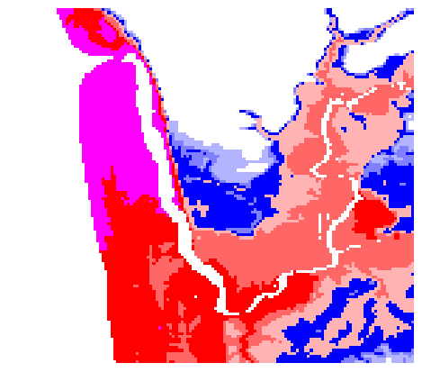
# colormap for depth h onshore and surface eta offshore:
bounds_depth_eta = array([1e-6,1,2,5,10,15,20])

cmap_depth_eta = mpl.colors.ListedColormap([[.7,.7,1],[.5,.5,1],[0,0,1],
                 [1,.7,.7], [1,.4,.4], [1,0,0]])

# Set color for value exceeding top of range to purple:
cmap_depth_eta.set_over(color=[1,0,1])

# Set color for land points without inundation to transparent if on image:
cmap_depth_eta.set_under(color=[0,0,0,0])

norm_depth_eta = mpl.colors.BoundaryNorm(bounds_depth_eta, cmap_depth_eta.N)
# temporary directory for files, which will be deleted at end:
kml_dir = os.path.join(os.getcwd(), 'kmlfiles')
print('Will send kml file and plots to kml_dir = \n  ', kml_dir)
os.system('mkdir -p %s' % kml_dir);

onshore = fgmax.B0 > 0
h_onshore = where(onshore, fgmax.h, nan)
eta_offshore = ma.masked_where(onshore, fgmax.h+fgmax.B0)

h_wet_onshore = ma.masked_where(h_onshore==0., h_onshore)
#print('fgmax.x, fgmax.y shapes: ',fgmax.x.shape, fgmax.y.shape)
#print('+++ h_wet_onshore.shape = ',h_wet_onshore.shape)
png_filename=kml_dir+'/h_onshore_max_for_kml.png'
fig,ax,png_extent,kml_dpi = kmltools.pcolorcells_for_kml(fgmax.X, fgmax.Y,
                                                 h_wet_onshore.T,
                                                 png_filename=png_filename,
                                                 dpc=2, cmap=cmap_depth_eta, norm=norm_depth_eta)
Will send kml file and plots to kml_dir =
   /home/runner/work/geoclaw_tsunami_tutorial/geoclaw_tsunami_tutorial/GTT/CopalisBeach/example2/kmlfiles
Using kml_dpi = 64,figure size 4.500000 by 3.937500 inches
Figure has 144 by 126 grid cells of uniform color
Dots per cell in x: 2.000000,  in y: 2.000000
       These should be integers
Created  /home/runner/work/geoclaw_tsunami_tutorial/geoclaw_tsunami_tutorial/GTT/CopalisBeach/example2/kmlfiles/h_onshore_max_for_kml.png
Convert the png extent to the format needed by folium#
x1,x2,y1,y2 = png_extent
image_bounds = [[y1,x1], [y2,x2]]
xc = (x1+x2)/2
yc = (y1+y2)/2
image_bounds
[[np.float64(47.11), np.float64(-124.19500000000001)],
 [np.float64(47.14500002800057), np.float64(-124.15499967999934)]]
Make an interactive folium map#
tiles = 'OpenStreetMap'  # default tiles
#tiles = 'OpenTopoMap'   # show contours

m = folium.Map(location=(yc, xc), tiles=tiles, zoom_start=13)

# Add the saved image as an overlay
folium.raster_layers.ImageOverlay(
    image='kmlfiles/h_onshore_max_for_kml.png',
    bounds=image_bounds,
    opacity=0.7, # Adjust opacity as needed
    name='Max Depth Onshore'
).add_to(m)

# Add a layer control to toggle the overlay
folium.LayerControl().add_to(m)

m
Save as an interactive html file#
You can save this map as an html file that can be posted on the web for any viewer to interact with, or embedded in a webpage as is done on the page Sample fgmax results.
m.save('folium_map_with_max_depth.html')