
Make ASCE_SIFT_Region2 dtopo file#
This Jupyter notebook is available in $GTT/dtopo/ASCE_SIFT_Region2.ipynb within the
GeoClaw Tsunami Tutorial.
It creates the file $GTT/dtopo/dtopofiles/ASCE_SIFT_Region2.dtt3, which can be used as a dtopofile in GeoClaw.
This particular tsunami source was created to produce a tsunami that satisfies certain requirements set out in the American Association of Civil Engineer’s (ASCE) guidelines for constructing certain critical infrastructure in tsunami inundation zones, as described in [WTT+17]. We use it here because it is easy to generate using the GeoClaw dtopotools module, since it is formed from the NOAA “SIFT unit sources” [GST+08].
See also
Rather than building this dtopofile, it is also possible to download it using GTT/dtopo/fetch_ASCE_SIFT_Region2.py.
Setup notebook and environment:#
%matplotlib inline
from pylab import *
from clawpack.geoclaw import dtopotools, topotools, kmltools
Load shoreline for plotting:#
This file was created with the Download etopo22 topography notebook.
csz_shore = loadtxt('../topo/topofiles/csz_shore.txt')
Create a fault using the NOAA SIFT database#
This particular fault is specified in terms of the NOAA SIFT unit sources, so we can use the clawpack.geoclaw.dtopotools.SiftFault class, which takes as an argument a dictionary sift_slip specifying the unit sources to be used and the slip on each.
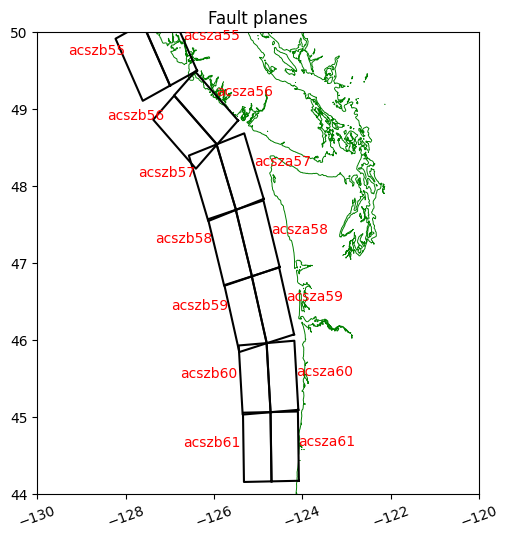
First we plot some of the unit sources on the CSZ margin.
f = dtopotools.SiftFault()
SIFT = f.sift_subfaults
sift_slips = {}
for k in SIFT.keys():
    s = SIFT[k]  # subfault
    s.longitude = s.longitude - 360.
    if (-130 <=s.longitude <= -120) and (44 <= s.latitude <= 50):
        if (k[4] in ['a','b']):
            sift_slips[k] = 0.
Downloading data from 'http://sift.pmel.noaa.gov/ComMIT/compressed/info_sz.dat' to file '/home/runner/.cache/pooch/2d12c2967b841187200a62a1ef69fbea-info_sz.dat'.
csz = dtopotools.SiftFault(sift_slips)
for k in sift_slips.keys():
    s = csz.sift_subfaults[k]  # subfault
    s.longitude = s.longitude - 360.

figure(figsize=(6,6))
ax = axes()
ax.plot(csz_shore[:,0], csz_shore[:,1], 'g', linewidth=0.7)
#axis([-140,-110,43,50])
ax.set_xlim(-130,-120)
ax.set_ylim(44,50)
csz.plot_subfaults(axes=ax)
ax.set_aspect(1./cos(55*pi/180.))

for k in sift_slips.keys():
    s = csz.sift_subfaults[k]  # subfault
    if k[4] == 'a':
        text(s.longitude, s.latitude, k, color='r')
    else:
        text(s.longitude-2, s.latitude, k, color='r')
Set the slip on a set of SIFT subfaults for this event#
event = 'ASCE_SIFT_Region2'
Slips provided by Yong Wei: 35ac57a+35ac57b+10ac58a+33ac58b+10ac59a+24ac59b+30ac60a+30ac60b
sift_slips = {'acsza57':35, 'acszb57':35 , 'acsza58':10 , 'acszb58':33 , 'acsza59':10 , 'acszb59':24 ,
              'acsza60':30 , 'acszb60':30 }
fault = dtopotools.SiftFault(sift_slips)
for k in sift_slips.keys():
    s = fault.sift_subfaults[k]  # subfault
    s.longitude = s.longitude - 360.
Create a uniform grid on which to evaluate the vertical deformation#
The grid spacing will be 10 arcseconds, with a buffer of 1 degree around the horizontal extent of the subfaults. (You could specify x,y to be any other desired points to define the deformation grid.)
x,y = fault.create_dtopo_xy(dx=10./3600., buffer_size=1)
print('Created uniform grid with %i points in x and %i in y' \
        % (len(x), len(y)))
Created uniform grid with 1801 points in x and 2161 in y
Apply the Okada model to each of the subfaults#
Okada applied to each subfault, with the specified slip, gives a vertical deformation that is evaluated at all points on the grid defined by x, y. These are added together for all the subfaults, since the Okada model is linear.
print('Creating dtopo by applying Okada model to %s subfaults...' % len(fault.subfaults))
dtopo_SIFT = fault.create_dtopography(x,y, verbose=False)
Creating dtopo by applying Okada model to 8 subfaults...
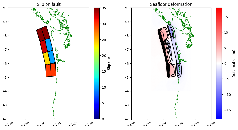
Plot the slip distribution and the resulting vertical deformation dz#
# for setting color scale:
dz_max = abs(dtopo_SIFT.dZ).max()
print("maximum abs(dz) over the full rupture time:", \
    abs(dtopo_SIFT.dZ).max())

fig = figure(figsize=(12,6))
ax1 = fig.add_subplot(121)
ax2 = fig.add_subplot(122)
fault.plot_subfaults(axes=ax1, slip_color=True)
dtopo_SIFT.plot_dZ_colors(axes=ax2, t=1, cmax_dZ=dz_max)

ax1.plot(csz_shore[:,0], csz_shore[:,1], 'g', linewidth=0.7)
ax1.set_xlim(-130,-120)
ax1.set_ylim(42,50)
ax1.set_aspect(1./cos(55*pi/180.))

ax2.plot(csz_shore[:,0], csz_shore[:,1], 'g', linewidth=0.7)
ax2.set_xlim(-130,-120)
ax2.set_ylim(42,50)
ax2.set_aspect(1./cos(55*pi/180.));

fname = 'dtopofiles/%s.png' % event
savefig(fname, bbox_inches='tight')
print('Created ',fname)
maximum abs(dz) over the full rupture time: 17.93480928266853
Created dtopofiles/ASCE_SIFT_Region2.png
Save as a dtopo file#
fname = 'dtopofiles/%s.dtt3' % event
dtopo_SIFT.write(fname, dtopo_type=3)
print('Created ',fname)
Created dtopofiles/ASCE_SIFT_Region2.dtt3
Make a kmz file that shows contours of dtopo:#
fname_kmz = 'dtopofiles/%s_contours.kmz' % event

kmltools.dtopo_contours2kmz([fname], dtopo_type=3,
                            dZ_interval=2, dZmax=20,
                            text_label=True,
                            text_x=dtopo_SIFT.x.min(),
                            text_y=dtopo_SIFT.y.mean(),
                            fname_kmz=fname_kmz)
Making contours for event =  ASCE_SIFT_Region2
  contour interval = 2m
Using kml_dpi = 576,figure size 12.506944 by 15.006944 inches
Figure has 1801 by 2161 grid cells of uniform color
Dots per cell in x: 4.000000,  in y: 4.000000
       These should be integers
Extent:   -127.570423  -122.567645   44.030951   50.033729
Created  dtopo_contours.kml
Created dtopofiles/ASCE_SIFT_Region2_contours.kmz
Removing  temp_dtopos_kml
Open the resulting file dtopofiles/ASCE_SIFT_Region2_contours.kmz in Google Earth to see contours of the vertical deformation.