
Comparison using the MOST model setup#
From the GeoClaw Tsunami Tutorial
See CopalisBeach examples for more about the Copalis Beach location and a list of other examples and tutorials based on this location.
This directory $GTT/CopalisBeach/MOST_comparison
contains code to perform a GeoClaw simulation that mimics the setup of
the MOST model used by the NOAA Center for Tsunami Research (NCTR),
which uses fixed nested grids at 3 resolutions, called the A, B, and C grids.
The Copalis Beach example used in this tutorial has also been explored by
the NCTR group using the MOST model, and they provided the grid data
that is in the subdirectory MOST_data. Note that these grids are used
both as the topography DEMs and as the computational grids in MOST.
(Use the fetch_MOST_data.py script to fetch this data.)
The script convert_most_to_asc.py converts these into a standard GeoClaw
topofile format for use as topofiles in this example.
The setrun.py file specifies 4 levels of fixed refinement with no regridding.
Levels 2, 3, 4 cover the same regions as the A, B, and C grids.
The coarsest Level 1 is a larger computational domain that is the same
size as used in example1 and exercise1, at the same 4 arcminute
resolution. This larger domain is added in order to capture
the outgoing portion of the initial waves without artifacts coming
from the domain boundaries. MOST handles this by using a precomputed
tsunami from the NOAA propagation database to provide boundary conditions
at the edge of the A grid.
If we omit this level and set the computational domain to be only the extent
of the A grid, then the initial waves approaching shore are accurate but the
simulation is soon contaminated by boundary effects.
Changes to setrun.py#
The file $GTT/CopalisBeach/exercise1/setrun.py
was modified to create the setrun.py file in this directory.
Below are the changes needed to force fixed resolution on the A, B, and C grids.
AMR levels#
The full domain and Level 1 resolution is the same as in exercise1.
We specify three additional levels of AMR with the resolutions of the
A, B, and C grids:
# max number of refinement levels:
amrdata.amr_levels_max = 4

# List of refinement ratios at each level (length at least mxnest-1)

# dx = dy = 4', 15", 3", 1/3"
refinement_ratios = [16,5,9]
amrdata.refinement_ratios_x = refinement_ratios
amrdata.refinement_ratios_y = refinement_ratios
amrdata.refinement_ratios_t = refinement_ratios
Forcing fixed refinement rather than adaptive#
We also specify that the initial grid refinement determined at time t0
should never be modified (no regridding is done), and that
the points flagged for refinement by the flagregions specified below
should not be buffered by additional points, so the refinement patches
at Levels 2 and 3 should identically agree with the B and C grids at all
times:
# steps to take on each level L between regriddings of level L+1:
amrdata.regrid_interval = 100000000  # NEVER REGRID

# width of buffer zone around flagged points:
# (typically the same as regrid_interval so waves don't escape):
amrdata.regrid_buffer_width  = 0   # NO BUFFER around Agrid, Bgrid, Cgrid

# clustering alg. cutoff for (# flagged pts) / (total # of cells refined)
# (closer to 1.0 => more small grids may be needed to cover flagged cells)
amrdata.clustering_cutoff = 0.7 # SHOULDN'T MATTER (only flag in rectangles)
Finally, the flagregions below specify four regions with each
spatial_region specified based on the extent of the domain and the
A, B and C grids. In each case minlevel = maxlevel is set to the desired
AMR level on this grid, imposing exactly this level of refinement.
# ---------------
# REGIONS:
# ---------------

flagregions = rundata.flagregiondata.flagregions  # empty list initially

# Computational domain:
flagregion = FlagRegion(num_dim=2)
flagregion.name = 'Region_domain'
flagregion.minlevel = 1
flagregion.maxlevel = 1
flagregion.t1 = 0.
flagregion.t2 = 1e9
flagregion.spatial_region_type = 1  # Rectangle
x1,y1 = clawdata.lower
x2,y2 = clawdata.upper
flagregion.spatial_region = [x1,x2,y1,y2]
flagregions.append(flagregion)


# MOST A grid:
flagregion = FlagRegion(num_dim=2)
flagregion.name = 'Region_Agrid'
flagregion.minlevel = 2
flagregion.maxlevel = 2
flagregion.t1 = 0.
flagregion.t2 = 1e9
flagregion.spatial_region_type = 1  # Rectangle
flagregion.spatial_region = [-126, -123.75, 45, 48.5]
flagregions.append(flagregion)

# MOST B grid
flagregion = FlagRegion(num_dim=2)
flagregion.name = 'Region_Bgrid'
flagregion.minlevel = 3
flagregion.maxlevel = 3
flagregion.t1 = 0.
flagregion.t2 = 1e9
flagregion.spatial_region_type = 1  # Rectangle
flagregion.spatial_region = [-126.5, -124.1, 47.0, 47.4]
flagregions.append(flagregion)

# MOST C grid
flagregion = FlagRegion(num_dim=2)
flagregion.name = 'Region_Cgrid'
flagregion.minlevel = 4
flagregion.maxlevel = 4
flagregion.t1 = 0.
flagregion.t2 = 1e9
flagregion.spatial_region_type = 1  # Rectangle
flagregion.spatial_region = [-124.25, -124.14, 47.1, 47.18]
flagregions.append(flagregion)
topofiles#
In addition to the topofiles provided by the MOST A, B, and C grids, we also
need a topofile that covers the larger computational domain, and for this
we use the same topofile as used in exercise1 and the other examples:
# 30-sec topo:
topo_file = f'{topodir}/etopo22_30s_-130_-122_40_50_30sec.asc'
topofiles.append([3, topo_file])
Note that this topofile is has 30” resolution, but the A grid topofile is at a 15” resolution and so it will take precidence in the region covered by the A grid (except where the finer B or C grids are used).
# A grid:
topo_file = f'{topodir}/Copalia_Agrid_15s_etopo2022.asc'
topofiles.append([3, topo_file])

# B grid:
topo_file = f'{topodir}/Copalis_Bgrid_3sec_mhw_13DEM_CUDEM_combine.asc'
topofiles.append([3, topo_file])

# C grid:
topo_file = f'{topodir}/copalis_Cgrid_10m_mhw.asc'
topofiles.append([3, topo_file])
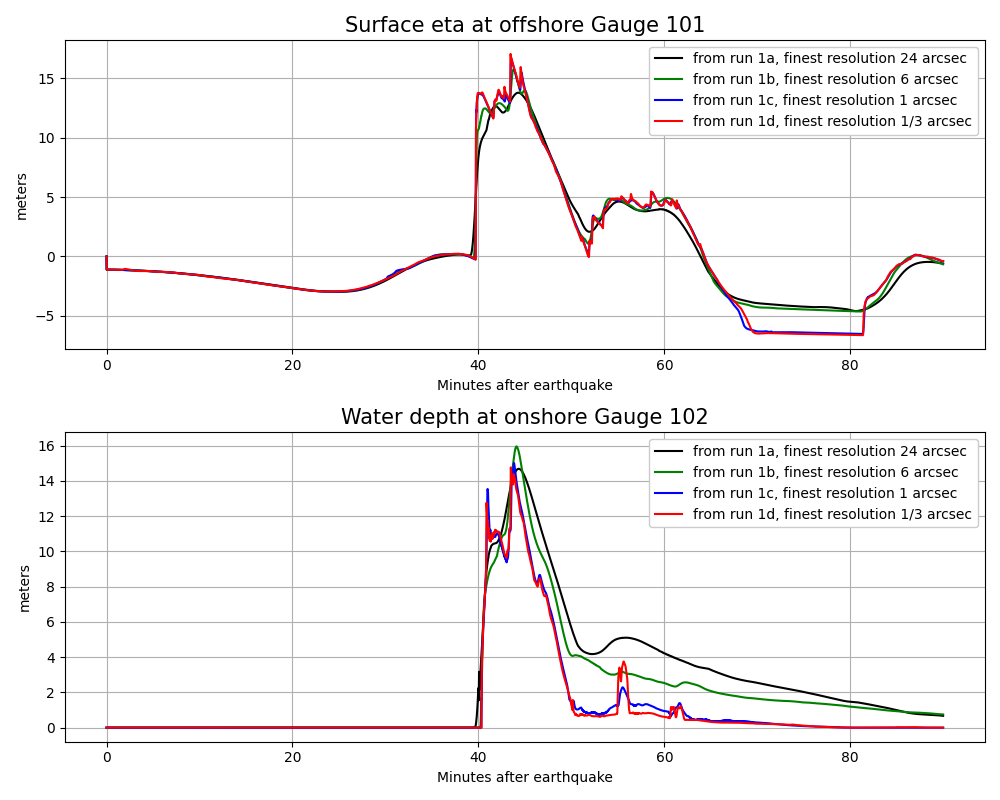
Computational results#
The final time for this simulation was set to tfinal = 1.5*3600.
and the finest level resolution is 1/3”, so the computational results should
be comparable to what was seen using setrun1d.py in example1.
The script compare_gauges.py produces plots of the time series
computed at the gauges for this comparison:
Note
This example is just to illustrate that fixed grid resolutions could be used if desired. Note that GeoClaw computes differently than MOST in many ways even if the grids are the same. For example:
Different numerical methods are used for solving the shallow water equations.
In GeoClaw the results computed on Level 3 are used to update the Level 2 grids whenever the times are synced up, and similarly at other levels, whereas in MOST the A grid computation is used to provide boundary data for the B grid, but its values are not updated by computations on the B grid.