Gauge plots for example1#
From the GeoClaw Tsunami Tutorial
The directory $GTT/CopalisBeach/example1
contains some initial GeoClaw setrun and setplot functions to start
exploring tsunami modeling.
See Copalis Beach example1 for more about these examples and Sample results for example1 for more discussion of the results obtained from 4 runs with different resolutions.
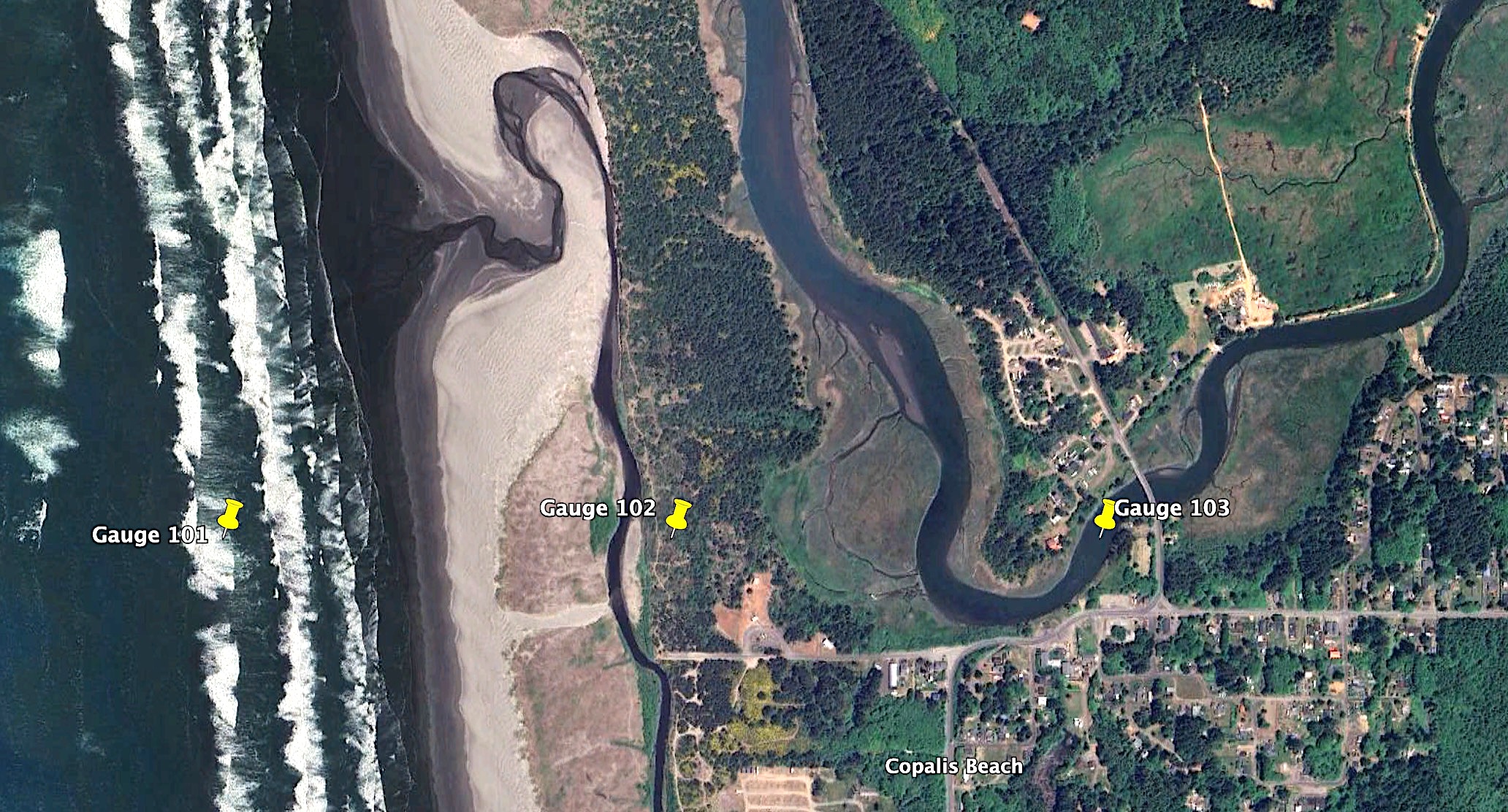
Gauge locations#
All of the setrun functions provided in this directory set the same 3
synthetic gauges via these lines:
gauges = rundata.gaugedata.gauges   # empty list initially

gauges.append([101, -124.1899537, 47.1159722, 0, 1e9])     # slightly offshore
gauges.append([102, -124.1800463, 47.1159722, 0, 1e9])     # onshore
gauges.append([103, -124.1706019, 47.1159722, 0, 1e9])     # in river
Note
Each gauge is specified by a list [gaugeno, x, y, t1, t2]
where t1 and t2 set the time interval over which the gauge will be
recording data, here from time 0 to “forever”.
The gauge locations x,y specified above have been chosen to be centered
in computational grid cells at the finest refinement levels used in this
problem. See centering_gauges for a description of why this is
desirable.
This centering is performed by the Python script center_gauges.py
in this directory.
The gauges.kml file created from any of these setrun files
shows the locations of the gauges specified:
Plots created by setplot.py#
The setplot.py files used for making plots from all four run cases
produces some crude gauge plots that you can find in the resulting
_PlotIndex.html within each of the plot directories (which are archived
in the sample_results directory).
Take a look at the gauge plots produced for case 1c (7 AMR levels with finest
resolution 1 arcsecond):
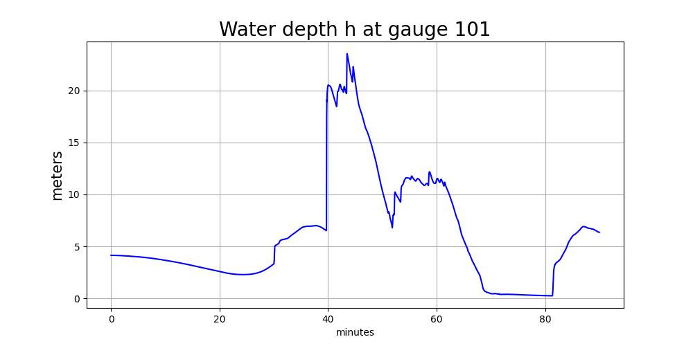
Gauge 101 offshore#
Here are plots of the water depth and surface elevation eta = h + B
at Gauge 101, which is just offshore (so there is initially water with depth h > 0
at time 0, seen from the depth plot below to be approximately 5 m).
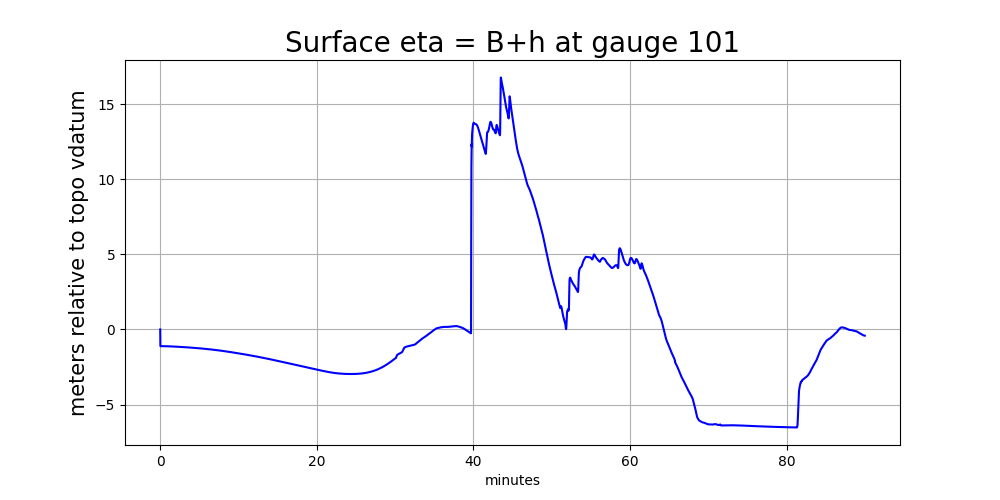
Note several things about these plots:
The surface elevation
eta = h + B(wherehis the water depth andBis the topography) is shown in meters relative to the vertical datum of the underlying topofileCopalis_13s.ascused in GeoClaw, since this is the finest-resolution topofile available at this gauge location (see TBD for more discussion of this). The way this topofile was created in Make topofiles for Copalis Beach, the vertical datum is (approximately) Mean High Water (MHW) at this location.The surface elevation plot shows a discontinuity in elevation just after time 0. This shows that this earthquake event has some co-seismic subsidence at the location of this gauge. As the land drops, the ocean drops with it and so the height of the jump discontinuity seen just after time 0 shows the magnitude of the subsidence at this location. (Add python code to show how this can be computed from gauge output).
The water depth plot does not show a discontinuity just after time 0. Since the land and ocean drop together due to the co-seismic deformation, there is no instantaneous change in the water depth at this point.
The main tsunami wave arrives at about 40 minutes, and both the surface elevation and water depth appear to rise almost discontinuously at this time. The shallow water equations we solve allow the formation of hydraulic jumps (shock waves) that roughly model the large bore that will be created when the huge leading wave of the tsunami shoals and breaks in the shallow water just offshore.
Before the main tsunami wave arrives, there is already some slower variations in the water level and surface elevation that correspond to a slow initial outflow of water (retreat of the shore line) followed by a small wave of elevation coming in. This is related to the offshore wave profile set up by the fact that this tsunami source has varying vertical deformation, with subsidence near shore (so the initial wave that arrives is a trough rather than a peak) with uplift farther offshore. (Modify Make ASCE_SIFT_Region2 dtopo file to show a transect of
dzat the latitude of Copalis Beach.)The earthquake event used here is an “instantaneous rupture” generated by the Okada model for the final vertical displacement of the seafloor and land after all the transient seismic waves have propagated away, and so the co-seismic deformation shows up as a jump discontinuity in
etajust aftert=0.Some tsunami models use a “kinematic rupture” source, e.g. computed by a 3D seismic model such as SPECFEM, based on specified time-dependent slips on the subfaults. In particular this was done for the new Cascadia CoPes Hub ground motions. (An example will be added later). Or, less frequently, a full “dyanamic rupture” source might be provided, as computed by a 3D code that models the rupture process itself from the stresses on the fault and strength of the rock. In either of these cases, the co-seismic deformation would not be instantaneous but would extend over the duration of the earthquake. Then the surface
etawould be seen to move up and down with the seismic waves over this time period. The water depthhwould still remain nearly constant over this time period, as the entire water column at this point moves up and down with the earthquake, but the horizontal variations in the vertical deformationdzwould also lead to small water waves starting to form over the same time period.
Discontinuities due to AMR level changes#
The water depth plot above also seems to show a discontinuity at about
30 minutes after the earthquake, a time at which the surface eta seems
to be smoothly varying. This discontinuity in h is totally non-physical and
is a spurious effect of the fact that we are using AMR and setrun1c.py
sets:
t_fine = 1800. # when to turn on finest level refinement (seconds)
and uses this to set
flagregion.t1 = t_fine
for the flagregions that control refinement to the finer AMR levels 6, 7,
and 8. So before 30 minutes, the nearshore area where Gauge 101 is located
is not allowed to be refined above Level 4, while after this time Level 7
is allowed. Note that in the setrun1c.py we set
amrdata.amr_levels_max = 7
so that the flagregion corresponding to Level 8 is never invoked.
(setrun1d.py sets amr_levels_max = 8 so see the plots in _plots1d
for that case.)
Each time regridding is performed when running GeoClaw, all of the gauges
are examined to see what the finest level grid patch is that includes that
gauge location. And then for every subsequent time step at this level,
a new gauge value is written out to the appropriate file in the _output
directory. (Or perhaps less frequently, if
gaugedata.min_time_increment is set, to be discussed elsewhere.)
See also
Also discussed elsewhere is whether the value is obtained by interpolation or just using the value in the finite volume cell that contains the gauge, see Nearshore Interpolation.
The level from which the gauge values were taken at each time are also
saved to the same gauge file in _output, and so we can examine these values.
A time series of the finest refinement level active around Gauge 101 is
also produced by setplot.py and looks like this (annotated by
the grid resolution at each level):
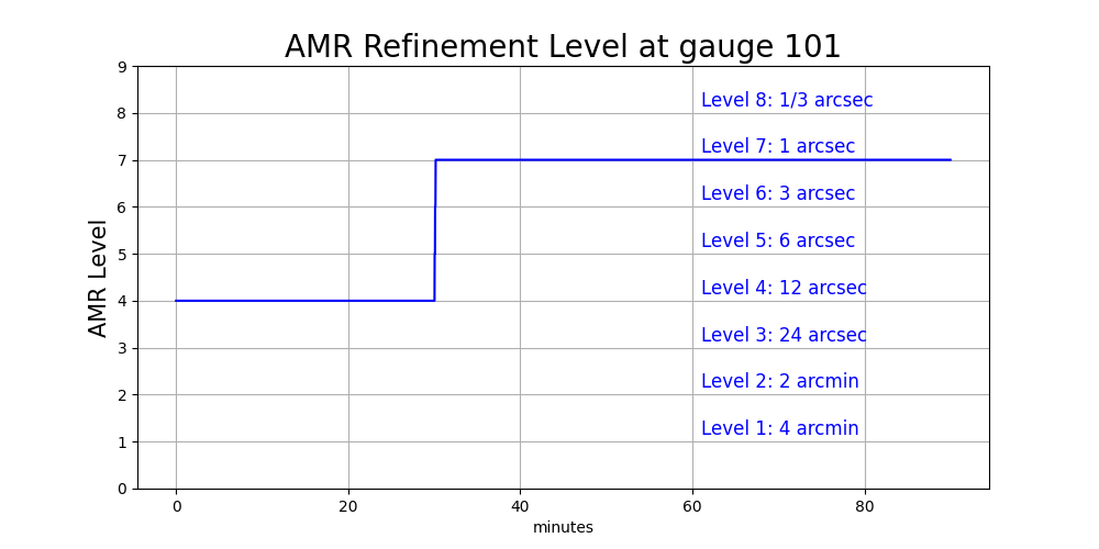
We clearly see the big jump from Level 4 to 7 at 30 minutes. When new grid
patches are introduced at a new AMR level, the topography B and water depth
h must be initialized for every grid cell in this patch. How is this done?
The value of B is computed in a grid cell by the process described in
more detail in ??, essentially integrating a piecewise bilinear
function defined by the finest available topofile(s) covering the cell over
the grid cell. Note that with the refinement factors specified in
setrun1c.py,
refinement_ratios = [2,5,2,2,2,3,3]
each cell at level 4 will be covered by 2x2 = 4 cells at level 5 and each
of those cells will be covered by 2x2 = 4 cells at level 6 and each
of those cells will be covered by 3x3 = 9 cells at level 7. And hence
a level 4 grid cell is covered by 4x4x9 = 144 cells at level 7. The sudden
refinement from level 4 to 7 results in much better resolution of the area
around Gauge 101, which now lies in one of the 144 cells covering the original
Level 4 grid cell it lies in.
Todo
More discussion of this…
Plots showing the topography B, h, and eta together#
The python script plot_gauge_h_eta.py produces some plots that may
help better understand how things behave when the mesh is refined around
a gauge.
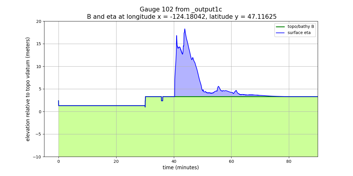
This plot shows the topography B as a green curve (filled with green below)
and the water surface eta as a blue curve (with the water between B and
eta also filled with blue, so the depth h at any time is the height of
this blue zone):
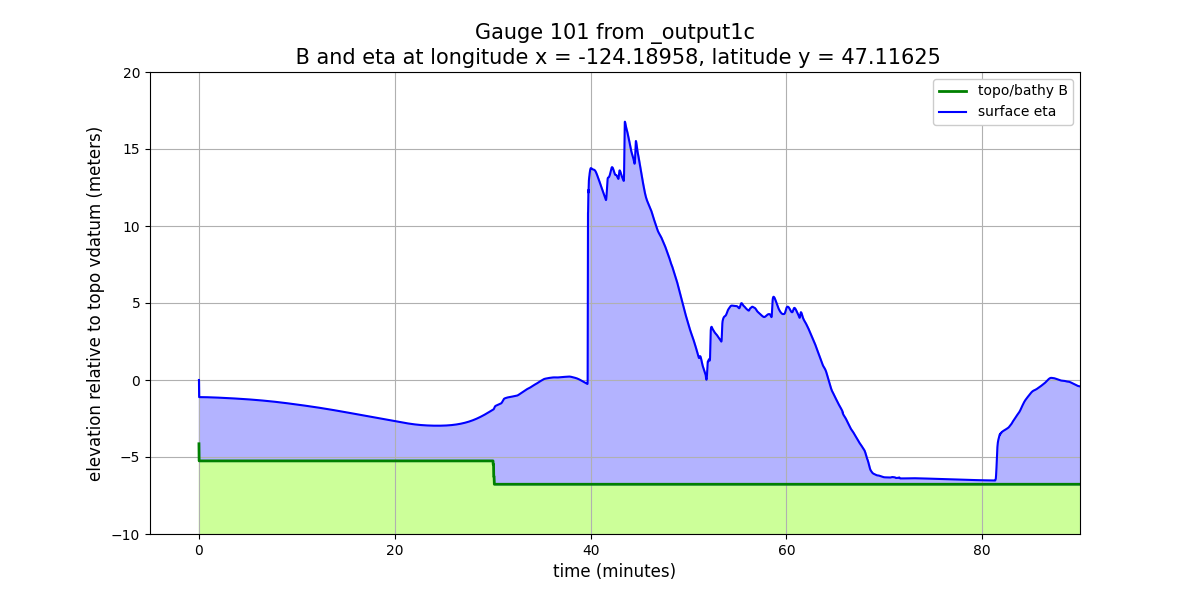
Again these are time series, and they show:
Just after time 0 there is a simultaneous and instantaneous drop in both
Bandeta, but the water depth does not change.At time 30 minutes, there is a jump in
Bdue to AMR refinement and so Gauge 101 is now in a level 7 grid cell with a smaller cell-averagedBvalue than the level 4 grid cell it lies in. The water depth on the new finer grid patches was initialized so that the water surfaceetadid not change (which required filling the cell with more water (largerh) than the original level 4 cell).
Plots like this are only useful in fairly shallow water, so that the distance
between B and eta is not huge compared to the variations in eta that
we wish to see. (For a gauge out in the deep ocean, at 3000 m depth, say,
the variations in eta for a realistic tsunami, of a few meters at most,
would appear as a flat line for eta).
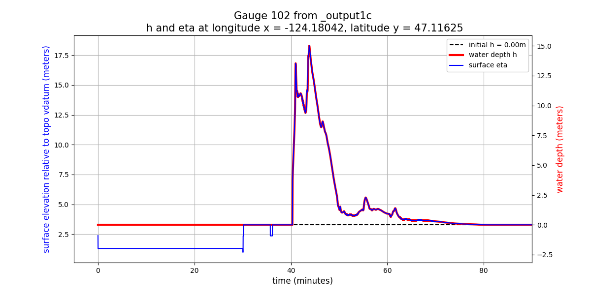
Another form of plot that is sometimes useful, particularly in deeper water,
is shown below. This shows h and eta on the same plot, but with different
vertical scales as shown on the left and right vertical axes:
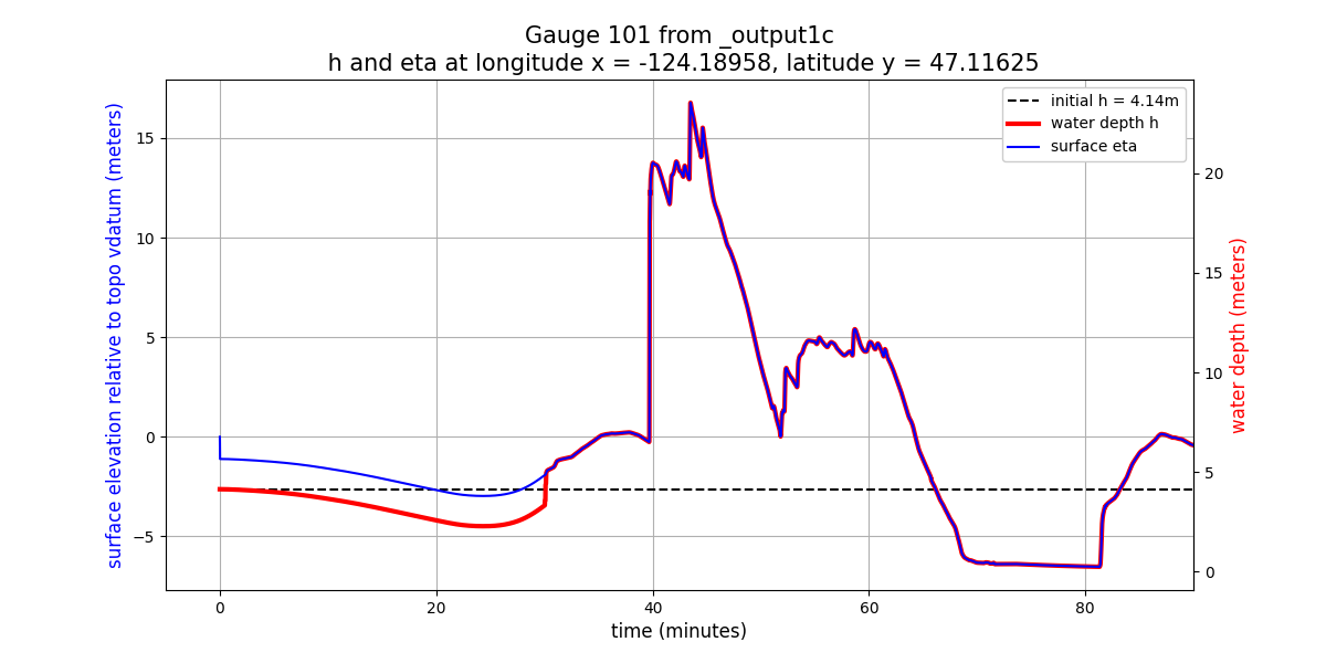
The offset between the h and eta scales was chosen so that the plots lie
on top of each other at the final time, and in fact they do so for all times
after 30 minutes (since the resolution does not change after that time
and so B = eta - h is constant in time).
But before 30 minutes there is an offset between the two due to the fact
that B was different on the coarser grid.
Also note that the co-seismic deformation just after time 0 shows up only
in eta and not in h.
Gauge 102 onshore#
Here are plots of the water depth and surface elevation eta = h + B
at Gauge 102, which is onshore (so there is initially no water at this
point at time 0).
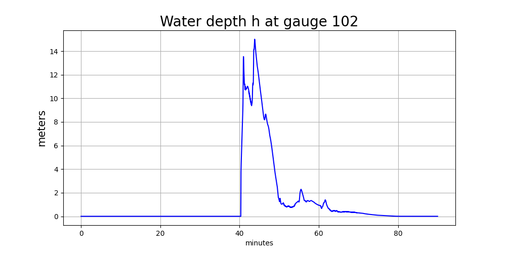
At this onshore location, the depth plot looks fine, starting a h=0 and
changing only when the tsunami arrives at this location
(as a nearly-discontinuous hyraulic jump).
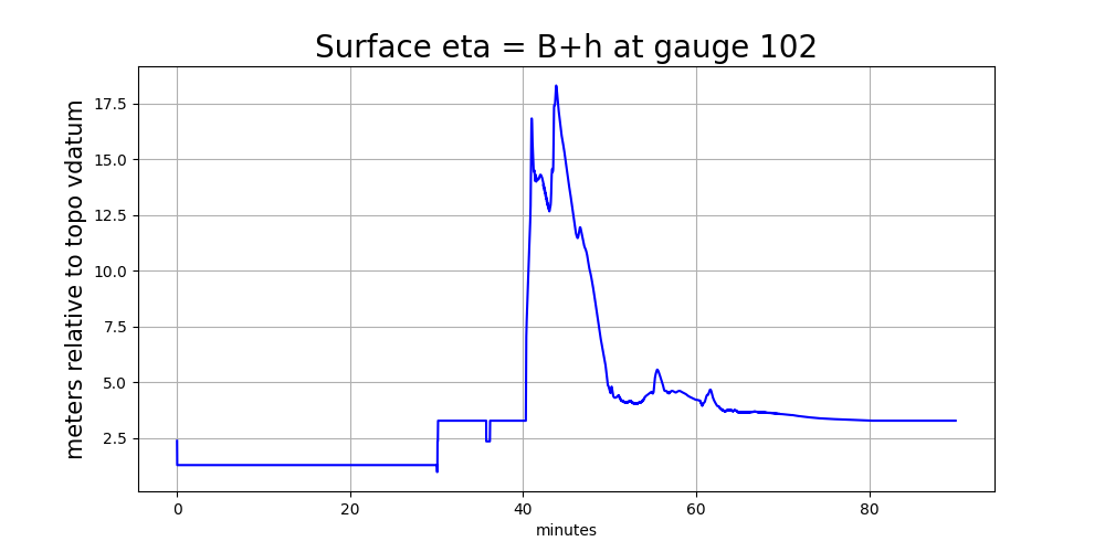
On the other hand the eta plot shows a discontinuity at 30 minutes and
some strange oscillations around 36 minutes. On dry land, h = 0 and so
eta = h + B = B is simply showing the topography value B at the gauge
location. At 30 minutes we refined from level 4 to 7 and so there was a
big jump in B in the finest-level grid cell covering Gauge 102.
This is the same discontinuity that shows up in the plots at the offshore
Gauge 101, but note that onshore it shows up in eta whereas offshore
it shows up in h.
The later oscillations in eta = B in the plot above are because after
refining to level 7 the simulation did not continue to use 7 levels at all
later times around the gauge location, as seen in this time series plot
of the AMR level at this gauge:

This oscillation in level is because this refinement
is controlled by a variable-level flagregion in setrun1c.py:
# Level 7 is 1 sec
flagregion = FlagRegion(num_dim=2)
flagregion.name = 'Region_1sec'
flagregion.minlevel = 5
flagregion.maxlevel = 7
flagregion.t1 = t_fine
flagregion.t2 = 1e9
flagregion.spatial_region_type = 1  # Rectangle
flagregion.spatial_region = [-124.25,-124.12,47.05,47.2]
flagregions.append(flagregion)
The gauges lie in the spatial_region specified here, but since
flagregion.minlevel = 5 it is not forcing 7 levels of refinement at this
point, only 5 levels (with a maximum of flagregion.maxlevel = 7).
What level it actually uses depends on how the solution is behaving around
this point at each refinement time (explain this better elsewhere).
Since water does not reach Gauge 102 until about 40 minutes, it does not
really need to refine to this level until just before that time.
(Why it refines to 7 levels much earlier and then oscillates between 6
and 7 levels needs more discussion.)
Here are the other plots we looked at above, now for the onshore Gauge 102:
Tip
In practice you might want to:
Choose between plotting
etaorhdepending on whether the gauge location is initial wet or dry.Create plots that only show times after which the refinement levels are no longer changing, typically the most interesting time anyway, after the tsunami arrives.
Set the time at which gauges are being recorded to the time you think the interesting behavior will start. In
setrun1c.pywe set the gauges as e.g.gauges.append([101, -124.1899537, 47.1159722, 0, 1e9])
This says that Gauge 101 is at lon-lat location
(-124.1899537, 47.1159722)and should be recording data from time0.to1e9(i.e. for the entire simulation no matter how largetfinalis, since1e9is essentially infinite). For the simulation shown here, it might be better to replace the start time0by38*60.for example, to only record gauges after 38 minutes.Set refinement
flagregionsto force refinement to the highest level after some time to insure you are not seeing spurious artifacts of level switching. You might also setflagregion.t1to an earlier time, so that the finest levels are present well before the interesting time at this location, and do not change thereafter.These changes might make the code run slower (by requiring refinement of regions where it’s never needed, such as farther onshore, or by refining long before the wave arrives), but in some cases may be well worth it to reduce confusion (e.g. when doing the final “production run” for a tsunami hazard assessment project).
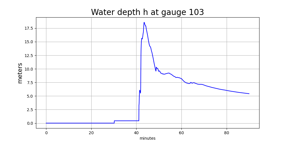
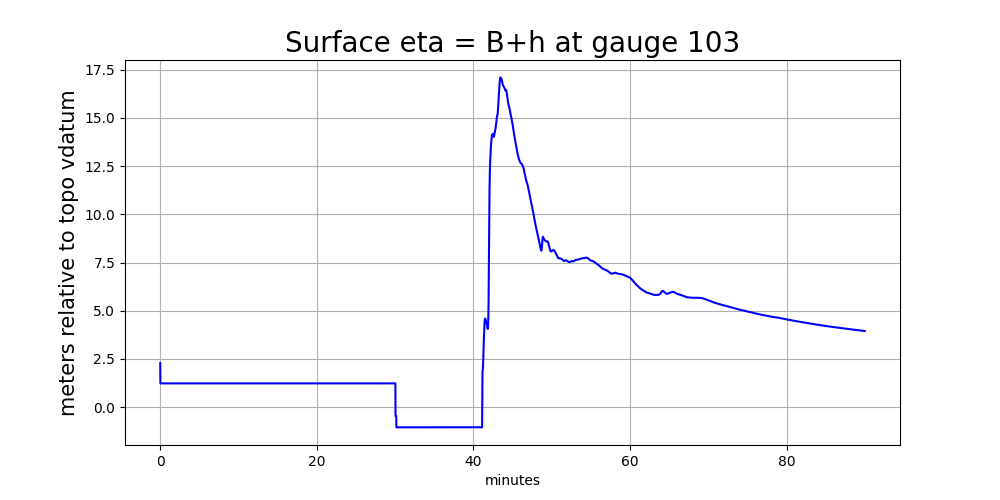
Gauge 103 in river#
Todo
Add discussion of what happens when gauge is on initially-dry land on coarse
levels but in an initially-wet cell on finer levels. This leads to
discontinuities in both h and eta at 30 minutes…