Plot fgout results#
This Jupyter notebook is available in $GTT/GTT/CopalisBeach/example2/plot_fgout.ipynb within the
GeoClaw Tsunami Tutorial.
See Copalis Beach example2 for details on the this simulation and the way the fgout grid was specified in setrun.py.
Before running this notebook, you must either run the GeoClaw simulation or else download the sample_results directory from the data repository. Note that this version of the code creates an output directory that only has the fgmax and fgout files needed for illustrating ways of plotting these results, without any full AMR time frame solutions (which would be much larger).
See also
Sample fgout results: for more discussion of fgout plots.
make_fgout_animation.py: script to make an animation of fgout results.
%matplotlib inline
from pylab import *
import os
from clawpack.geoclaw import fgout_tools
from clawpack.visclaw import geoplot, gridtools, plottools
if 1:
    # use this to fetch sample_results from the online data repository:
    if not os.path.isdir('sample_results'):
        import fetch_sample_results
    outdir = 'sample_results/_output'
else:
    # use this if you have run the code locally to create '_output'
    outdir = '_output'

output_format = 'binary32'  # should agree with setrun.py
Loading fgout results#
Before reading any frames, we read in the input data from fgout_grids.data that specify how the grid was defined.
fgno = 1   # fgout grid identifier

# Instantiate object for reading fgout frames:
fgout_grid = fgout_tools.FGoutGrid(fgno, outdir, output_format)

# Read the fgout input data that defines the grid:
fgout_grid.read_fgout_grids_data()
Reading fgout grid info from
    sample_results/_output/fgout_grids.data
Reading input for fgno=1, point_style = 2
Found fgout grid q_out_vars =  [1, 2, 3, 4]
Using this mapping to fgout variable names:
      qmap =  {'h': 1, 'hu': 2, 'hv': 3, 'eta': 4, 'B': 5}
Now we can read a single frame via, e.g.
fgframe = 20
fgout = fgout_grid.read_frame(fgframe)
Reading Frame 20 at t = 2940 from outdir = /home/runner/work/geoclaw_tsunami_tutorial/geoclaw_tsunami_tutorial/GTT/CopalisBeach/example2/sample_results/_output
The variables stored for each frame are h, hu, hv, eta, and these are all attributes of the fgout object created by reading a frame. fgout.B will also be computed automatically from fgout.h and fgout.eta and will be the topography at this output time. These arrays all have the same shape:
Attributes of fgout#
The fgout object created above has many attributes set, in particular:
fgout.x,fgout.y: 1D arrays of longitudes,latitudes at fgout pointsfgout.X,fgout.Y: 2D arrays with(X[i,j], Y[i,j])=(x[i],y[j])value at the(i,j)fgout pointfgout.h: 2D array ofhat each pointfgout.B: 2D array of topographyBat each point (at this fgout time)
print('fgout.x.shape = ', fgout.x.shape)
print('fgout.y.shape = ', fgout.y.shape)
print('fgout.B.shape = ', fgout.B.shape)
fgout.x.shape =  (144,)
fgout.y.shape =  (126,)
fgout.B.shape =  (144, 126)
Make a simple plot#
Now the fgout attributes can used to produce whatever plots you want.
The example below produces one plot similar to a single frame of
the animation produced by make_fgout_animation.py.
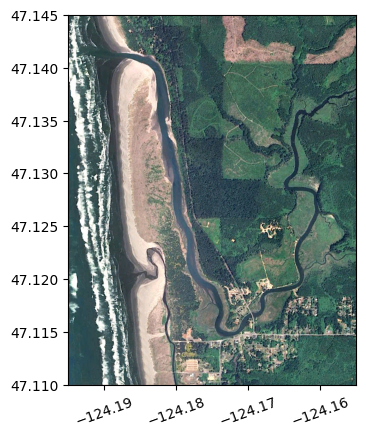
Load a background image#
This image was captured from Google Earth by opening fgout0001.kml and making a screenshot of the rectangular region shown.
fg_image = imread('fg_background.jpg')
fg_extent = [-124.195, -124.155, 47.11, 47.145]
imshow(fg_image, extent=fg_extent)

# fix axes:
ticklabel_format(style='plain',useOffset=False)
xticks(rotation=20)
gca().set_aspect(1./cos(47*pi/180.));  # adjust aspect ratio for this latitude
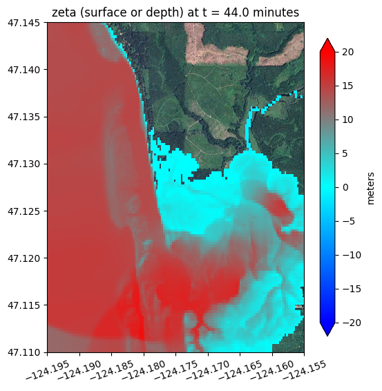
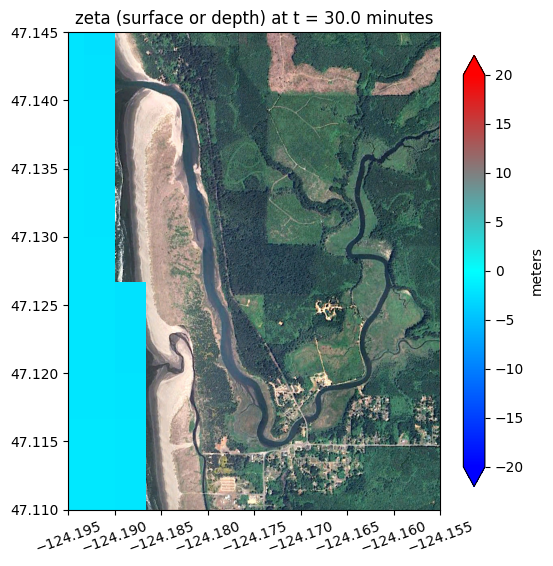
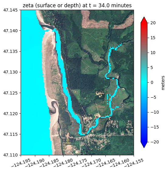
def plot_fgout_frame(fgframeno):
    """
    Load frame fgframeno of fgout data and produce a plot
    """

    # load frame:
    fgout = fgout_grid.read_frame(fgframeno)

    figure(figsize=(6,8))
    imshow(fg_image, extent=fg_extent)

    # Define zeta to be h onshore, h+B=eta offshore
    # Here we define onshore using the current fgout.B at each time

    onshore = fgout.B > 0
    zeta = where(onshore, fgout.h, fgout.h+fgout.B)
    zeta = ma.masked_where(fgout.h<0.01, zeta)

    plottools.pcolorcells(fgout.X, fgout.Y, zeta,
                                     cmap=geoplot.tsunami_colormap)

    clim(-20,20)
    colorbar(extend='both', shrink=0.7, label='meters')

    title(f'zeta (surface or depth) at t = {fgout.t/60} minutes')

    # fix axes:
    ticklabel_format(style='plain',useOffset=False)
    xticks(rotation=20)
    gca().set_aspect(1./cos(47*pi/180.));  # adjust aspect ratio for this latitude
Plot a few fgout frames:#
plot_fgout_frame(1)
Reading Frame 1 at t = 1800 from outdir = /home/runner/work/geoclaw_tsunami_tutorial/geoclaw_tsunami_tutorial/GTT/CopalisBeach/example2/sample_results/_output
plot_fgout_frame(5)
Reading Frame 5 at t = 2040 from outdir = /home/runner/work/geoclaw_tsunami_tutorial/geoclaw_tsunami_tutorial/GTT/CopalisBeach/example2/sample_results/_output
plot_fgout_frame(15)
Reading Frame 15 at t = 2640 from outdir = /home/runner/work/geoclaw_tsunami_tutorial/geoclaw_tsunami_tutorial/GTT/CopalisBeach/example2/sample_results/_output