Sample fgmax results#
From the GeoClaw Tsunami Tutorial
The directory $GTT/CopalisBeach/example2
contains a GeoClaw example that produces results on fgout and fgmax grids.
See also
Copalis Beach example2 for more about this example, and general discussion of fgout and fgmax grids.
Plot fgmax results is a Jupyter notebook that plots the fgmax results.
chile2010_fgmax-fgout shows results from the example included with GeoClaw in
$CLAW/geoclaw/examples/tsunami/chile2010_fgmax-fgout, which also illustrates how to make fgout animations, similar to what is described here, using the Chile 2010 event in the offshore region.
The script fetch_sample_results.py can be used to fetch some sample
results if you want to run the post-processing script or notebook in
this directory without running the GeoClaw code.
Reading and plotting fgmax results#
The notebook Plot fgmax results illustrates the basic approach to reading in fgmax results and producing various types of plots.
Creating kmz files to view on Google Earth#
The script make_fgmax_kmz.py creates a set of plots as png files with a
kml file wrapper that allows them to be overlaid on Google Earth. All the
files are combined into a self-contained kmz file, which is also available as
sample_results/CopalisBeach_ASCE_SIFT_fgmax1.kmz.
Producing and using this file allows you to zoom in on region of interest to
better explore the fgmax results.
The kmz file can also be uploaded to a project on earth.google.com so that others can also explore your fgmax results and interact via a webpage. The sample file produced in this example can be viewed at this link.
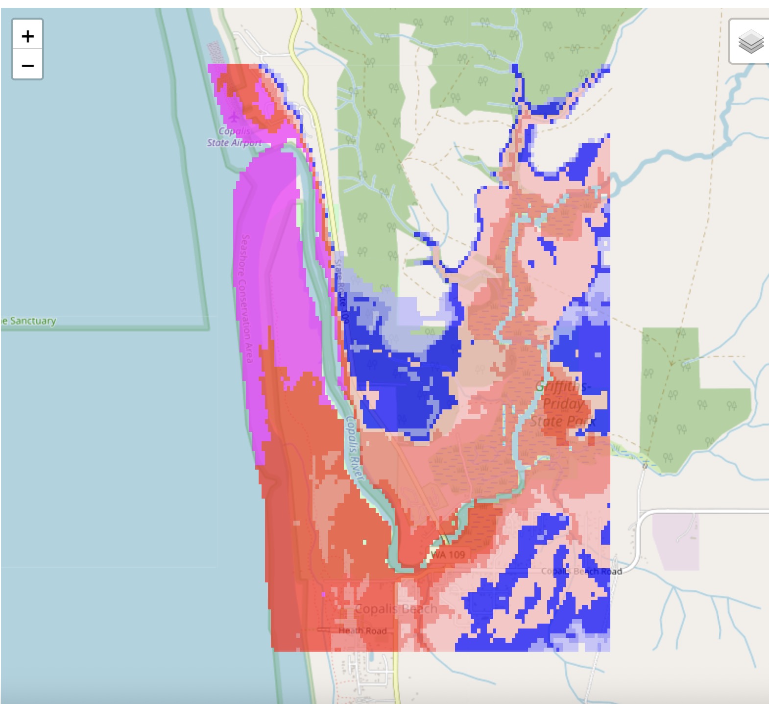
Plotting fgmax results on folium maps#
The notebook Plot fgmax results on an interactive map produces an intereactive plot of the maximum water depth on top of a leaflet.js map produced using the Python package folium.
Here is a screenshot, or see Interactive fgmax results for an interactive view.