Plot fgmax results for Copalis Beach example2

This Jupyter notebook is available in $GTT/GTT/CopalisBeach/example2/plot_fgmax.ipynb within the GeoClaw Tsunami Tutorial.

See Copalis Beach example2 for details on the this simulation and the way the fgmax grid was specified in setrun.py.

Before running this notebook, you must either run the GeoClaw simulation or else download the sample_results directory from the data repository. Note that this version of the code creates an output directory that only has the fgmax and fgout files needed for illustrating ways of plotting these results, without any full AMR time frame solutions (which would be much larger).

See also

• make_fgmax_kmz.py makes plots of the fgmax results with a wrapper to open them and view on Google Earth.

%matplotlib inline

from pylab import *
import os
from clawpack.geoclaw import fgmax_tools
from clawpack.visclaw import geoplot, gridtools, plottools

if 1:
    # use this to fetch sample_results from the online data repository:
    if not os.path.isdir('sample_results'):
        import fetch_sample_results  # fetches directory
    outdir = 'sample_results/_output'
else:
    # use this if you have run the code locally to create '_output'
    outdir = '_output'

Read fgmax results

fgmax = fgmax_tools.FGmaxGrid()

fgmax.outdir = outdir  # as set at top of this notebook

# read the input data used for this run:
data_file = os.path.join(fgmax.outdir, 'fgmax_grids.data')
fgmax.read_fgmax_grids_data(fgno=1, data_file=data_file)

# read fgmax results:
fgmax.read_output()

Reading input for fgno=1, point_style = 2 
Reading sample_results/_output/fgmax0001.txt ...

Attributes of fgmax

The fgmax object created above has many attributes set, in particular:

• fgmax.x, fgmax.y: 1D arrays of longitudes,latitudes at fgmax points

• fgmax.X, fgmax.Y: 2D arrays with (X[i,j], Y[i,j]) = (x[i],y[j]) value at the (i,j) fgmax point

• fgmax.h: 2D array of maximum h at each point

• fgmax.s: 2D array of maximum speed s at each point

print('fgmax.x.shape = ', fgmax.x.shape)
print('fgmax.y.shape = ', fgmax.y.shape)
print('fgmax.h.shape = ', fgmax.h.shape)

fgmax.x.shape =  (144,)
fgmax.y.shape =  (126,)
fgmax.h.shape =  (144, 126)

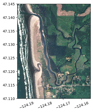
Load a background image

This image was captured from Google Earth by opening fgmax0001.kml and making a screenshot of the rectangular region shown.

fg_image = imread('fg_background.jpg')
fg_extent = [-124.195, -124.155, 47.11, 47.145]
imshow(fg_image, extent=fg_extent)

# fix axes:
ticklabel_format(style='plain',useOffset=False)
xticks(rotation=20)
gca().set_aspect(1./cos(47*pi/180.));  # adjust aspect ratio for this latitude

Recover the original pre-seismic topography

The fgmax data includes fgmax.B, the GeoClaw topography value at each fgmax point. However, these values were stored when the fgmax grid was first turned on at 35 minutes after the earthquake and so contains the subsidence of the coast that is included in the dtopo used for this example.

If we want to plot the original shoreline, or plot only the onshore inundation, then we need to adjust fgmax.B by this subsidence value to obtain B0, the initial topography.

One approach that is often used is to do a separate GeoClaw run with no dtopo file over a very short time period with the finest AMR resolutions and also the fgmax grid monitoring turned on immediately at time 0. The fgmax.B values from this run can then be used as the intial topography B0.

Here we take a simpler approach and interpolate from the dtopo file to the fgmax points to determine roughly the amount of subsidence at each fgmax point. This approach is built into the fgmax_tools.py module, so we can simply use the function fgmax.interp_dz as follows:

dtopodir = '../../dtopo/dtopofiles'
dtopofile = os.path.join(dtopodir, 'ASCE_SIFT_Region2.dtt3')
fgmax.interp_dz(dtopofile, dtopo_type=3)

Over fgmax extent, min(dz) = -1.14 m, max(dz) = -0.97 m

This shows that over the region covered by our fgmax grid, there is roughly 1 meter of subsidence.
This also sets fgmax.dz to the deformation at each fgmax point and we can subtract this from fgmax.B to get an estimate of the original topography:

fgmax.B0 = fgmax.B - fgmax.dz

print('The new attribute fgmax.B0 has the same shape as other arrays: ',fgmax.B0.shape)

The new attribute fgmax.B0 has the same shape as other arrays:  (144, 126)

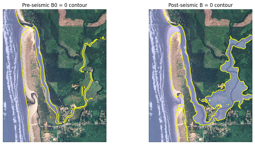
The plot below shows that this makes a significant difference in the shoreline position, with much of the Copalis River valley below MHW post-event.

figure(figsize=(12,6))
subplot(1,2,1)
imshow(fg_image, extent=fg_extent)
# color region below MHW light blue and semi-transparent:
contourf(fgmax.X, fgmax.Y, fgmax.B0, [-100., 0.], colors=[[.7,.7,1,0.5]])
# contour line at B0=0:
contour(fgmax.X, fgmax.Y, fgmax.B0, [0.], colors='yellow')
title('Pre-seismic B0 = 0 contour')
axis('off')
gca().set_aspect(1./cos(fgmax.Y.mean()*pi/180.));

subplot(1,2,2)
imshow(fg_image, extent=fg_extent)
contourf(fgmax.X, fgmax.Y, fgmax.B, [-100., 0.], colors=[[.7,.7,1,0.5]])
contour(fgmax.X, fgmax.Y, fgmax.B, [0.], colors='yellow')
title('Post-seismic B = 0 contour')
axis('off')
gca().set_aspect(1./cos(fgmax.Y.mean()*pi/180.));

Plotting fgmax results

After reading the fgmax object, there are several arrays that you can plot with any tools / colormaps you want. In particular, these 2D arrays are have the same shape:

• fgmax.X, fgmax.Y: longitude and latitude at each point

• fgmax.B, fgmax.B0: final and inital topography at each point (B0 was calculated above)

• fgmax.h, fgmax.s: maximum water depth and speed recorded at each point

What is “onshore”?

For some applications you might want to plot only the depth at points that are “onshore”. In this case we typically use the pre-seismic topography B0 to define what is meant by “onshore”. Points near the coast may no longer be onshore at MHW after subsidence, but for mapping purposes people want to see the water depth at points on the beach or near structures that start out onshore.

Plotting zeta

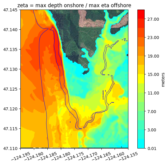
When plotting maxima for regions that include both onshore and offshore points, it is often useful to define a variable we call zeta that is defined to be the maximum h for onshore points (where people care about the water depth) and the maximum eta = h + B0 for offshore points (where the water depth may be huge in the ocean, and people care instead about disturbances in the surface elevation).

Defining zeta this way, as done in the next cell, also has the advantage that zeta is continuous at the (pre-seismic) shoreline where B0 = 0.

onshore = fgmax.B0 > 0
h_onshore = where(onshore, fgmax.h, nan)
zeta = where(onshore, fgmax.h, fgmax.h+fgmax.B0)

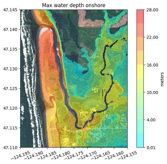
A couple sample plots

clines = [0.01] + list(arange(1,30,3))
nlines = len(clines)
n1 = int(floor((nlines-1)/2.))
n2 = nlines - 1 - n1
Green = hstack([linspace(1,1,n1),linspace(1,0,n2)])
Red = hstack([linspace(0,0.8,n1), ones(n2)])
Blue = hstack([linspace(1,0.2,n1), zeros(n2)])
Alpha = 0.5*ones(nlines)  # transparency
colors = list(zip(Red,Green,Blue,Alpha))

figure(figsize=(8,6))
imshow(fg_image, extent=fg_extent)

contourf(fgmax.X,fgmax.Y,h_onshore,clines,colors=colors)

colorbar(extend='max', label='meters')
title('Max water depth onshore')

# fix axes:
ticklabel_format(style='plain',useOffset=False)
xticks(rotation=20)
gca().set_aspect(1./cos(fgmax.Y.mean()*pi/180.));

clines_zeta = [0.01] + list(arange(1,30,2))
colors_zeta = geoplot.discrete_cmap_1(clines_zeta)

figure(figsize=(8,6))
imshow(fg_image, extent=fg_extent)
contourf(fgmax.X,fgmax.Y,zeta,clines_zeta,colors=colors_zeta)

colorbar(extend='max', label='meters')
contour(fgmax.X,fgmax.Y,fgmax.B0,[0.],colors='b', linewidths=0.7)
title('zeta = max depth onshore / max eta offshore')

# fix axes:
ticklabel_format(style='plain',useOffset=False)
xticks(rotation=20)
gca().set_aspect(1./cos(fgmax.Y.mean()*pi/180.));

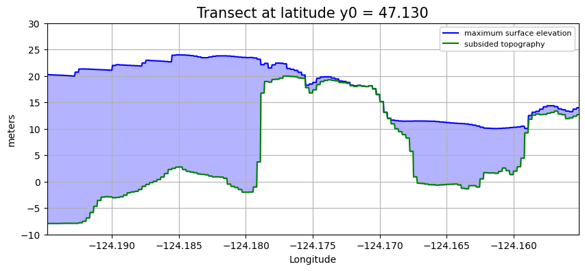
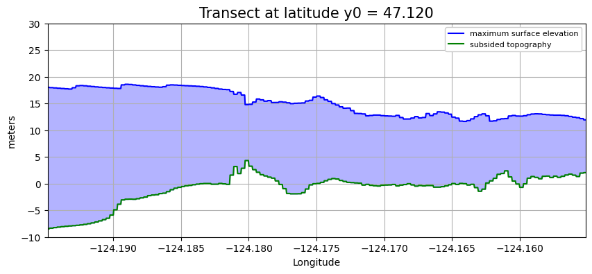
Transect plots

The clawpack.visclaw.gridtools module contains a function grid_eval_2d for extracting the solution along a transect from the 2D data in one of the fgmax arrays.

Here are a couple of sample transect plots:

def extract_transect(fgmax, xtrans, ytrans):
    h1d = gridtools.grid_eval_2d(fgmax.X, fgmax.Y,
                                   fgmax.h, xtrans, ytrans)
    B1d = gridtools.grid_eval_2d(fgmax.X, fgmax.Y,
                                 fgmax.B, xtrans, ytrans)
    return B1d, h1d

def plot_transect(y0):
    xtrans = linspace(fgmax.x.min(), fgmax.x.max(), 1000)
    ytrans = y0 * ones(xtrans.shape)
    B1d, h1d = extract_transect(fgmax, xtrans, ytrans)
    eta1d = B1d + h1d
    
    figure(figsize=(10,4))
    
    fill_between(xtrans, B1d, eta1d, color=[.7,.7,1])
    plot(xtrans, eta1d, 'b', label='maximum surface elevation')
    plot(xtrans, B1d, 'g', label='subsided topography')
    grid(True)
    ticklabel_format(useOffset=False)
    xlim(xtrans.min(), xtrans.max())
    ylim(-10, 30)
    xlabel('Longitude')
    ylabel('meters')
    legend(loc='upper right', framealpha=1, fontsize=8)
    title(f'Transect at latitude y0 = {y0:.3f}', fontsize=15);

plot_transect(y0=47.130)

plot_transect(y0=47.120)

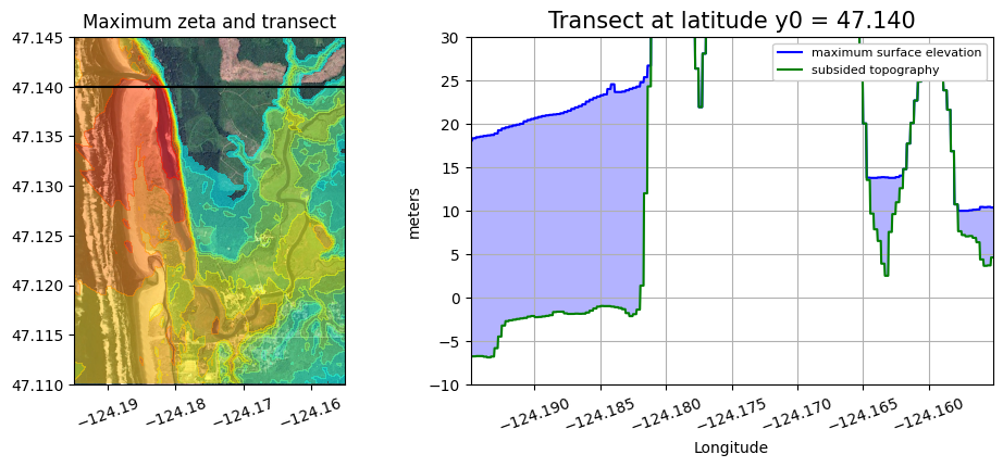
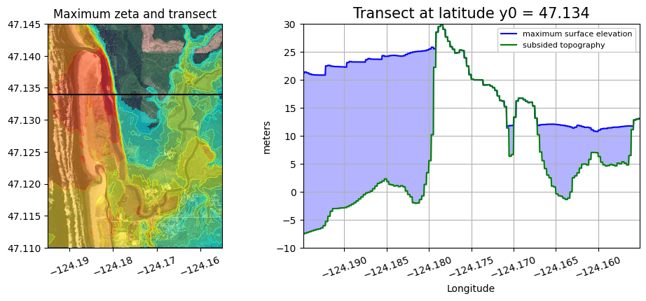
A version that also shows where the transect is in plan view

def plot_transect(y0):
    xtrans = linspace(fgmax.x.min(), fgmax.x.max(), 1000)
    ytrans = y0 * ones(xtrans.shape)
    B1d, h1d = extract_transect(fgmax, xtrans, ytrans)
    eta1d = B1d + h1d
    
    figure(figsize=(12,4))

    axes([.1,.1,.4,.8])
    imshow(fg_image, extent=fg_extent)
    contourf(fgmax.X,fgmax.Y,zeta,clines,colors=colors)
    plot(xtrans,ytrans,'k')
    ticklabel_format(style='plain',useOffset=False)
    gca().set_aspect(1./cos(fgmax.Y.mean()*pi/180.));
    xticks(rotation=20)
    title('Maximum zeta and transect')

    axes([.5,.1,.4,.8])
    fill_between(xtrans, B1d, eta1d, color=[.7,.7,1])
    plot(xtrans, eta1d, 'b', label='maximum surface elevation')
    plot(xtrans, B1d, 'g', label='subsided topography')
    grid(True)
    ticklabel_format(useOffset=False)
    xlim(xtrans.min(), xtrans.max())
    ylim(-10, 30)
    xlabel('Longitude')
    xticks(rotation=20)
    ylabel('meters')
    legend(loc='upper right', framealpha=1, fontsize=8)
    title(f'Transect at latitude y0 = {y0:.3f}', fontsize=15);

plot_transect(y0=47.134)

plot_transect(y0=47.140)