Sample results for example1

Sample results for example1#

The directory $GTT/CopalisBeach/example1 contains some initial GeoClaw setrun and setplot functions to start exploring tsunami modeling.

See Copalis Beach example1 for more about these examples.

Fetch the sample results#

The code cell hidden below runs fetch_sample_results.py to download the subdirectory sample_results that provides the figures shown on this page.

The setrun files defined in this directory are all nearly identical, but allow a different number of refinement levels. The coarsest (3-level) case runs quickly and shows how things are refined in most of the domain. The other versions add refinement levels only near Copalis Beach, and so the full domain plots look nearly identical and are not shown in the videos below.

See Setting up the GeoClaw run for detailed description of the setrun1a.py script, and Annotated screen output for more discussion of the output.

Run times#

Here’s a summary of some run times, but note that these may vary from run to run (even on the same computer), particularly for short runs.

These runs were done on a Macbook Pro with the M1 chip and 6 OpenMP threads.

example	finest-level grid resolution	elapsed wall time	Total CPU time
setrun1a	24 arcsec (level 3)	35 seconds	181 seconds
setrun1b	6 arcsec (level 5)	314 seconds	1716 seconds
setrun1c	1 arcsec (level 7)	465 seconds	2602 seconds
setrun1d	1/3 arcsec (level 8)	1780 seconds	10275 seconds

More details about the run time is summarized in a table that gets written to the timing.txt at the end of a run (this information is also printed to the screen). For example, here’s _output1d/timing.txt:

============================== Timing Data ==============================

Integration Time (stepgrid + BC + overhead)
Level           Wall Time (seconds)    CPU Time (seconds)   Total Cell Updates
  1                     1.241                  2.417            0.999E+06
  2                     2.487                  9.488            0.115E+08
  3                    36.296                190.706            0.271E+09
  4                   183.886               1077.718            0.170E+10
  5                    13.987                 62.963            0.950E+08
  6                    33.994                169.437            0.276E+09
  7                   192.710               1065.166            0.169E+10
  8                  1249.079               7478.786            0.116E+11
total                1713.681              10056.682            0.156E+11

All levels:
stepgrid             1673.687               9936.121    
BC/ghost cells         18.104                 98.417
Regridding             51.003                162.183  
Output (valout)         0.361                  0.341  

Total time:          1779.518              10275.146  
Using  6 thread(s)

Note: The CPU times are summed over all threads.
      Total time includes more than the subroutines listed above
Note: timings are also recorded for each output step
      in the file timing.csv.

Note that more than 15 billion grid cells were updated during this computation (counting each grid cell on every level for each time step on that level). You can also see that the majority of the work was done on the finest Level 8 grids.

You can also view plots of these timing results for the various runs from the link that shows up at the bottom of the _PlotIndex.html file in each _plots directory.

Here’s just one of the timing plots, from _plots1d for the finest level run:

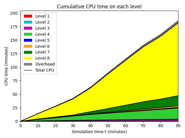
This shows the cumulative CPU time (which are collected in the file timing.csv in the _output directory at each output time, and for these runs output every 10 minutes was specified). Again we see that the majority of the work was done on Level 8. Note also the gray section above the yellow Level 8 section on the plot. This shows the amount of time spent on “overhead” related to the way the AMR is implemented. This cost of using AMR is tiny compared to the cost savings inherent in putting finer grids only where they are really needed!

Four _plots directories are created if you run the make_all.sh script, as described in Copalis Beach example1.

Note

Archived versions of all of these _plots directories are fetched to the sample_results directory if you run the fetch_sample_results.py script, as described in Copalis Beach example1, so that you can view them without needing to perform all the runs.

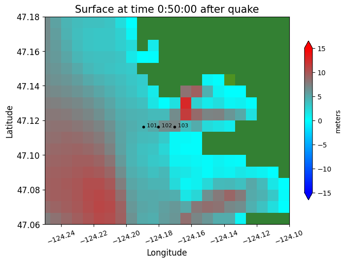
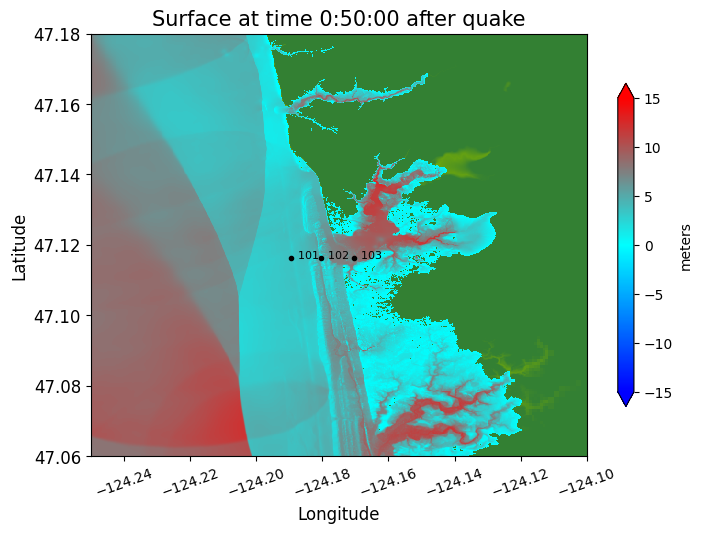
Comparison of the inundation#

Shown around Copalis Beach with different finest-level resolution, at time 50 minutes.

These plots also show the location of 3 gauges. See Gauge comparisons below for comparisons of time series at these gauges as computed with the different resolutions shown here.

24” resolution#

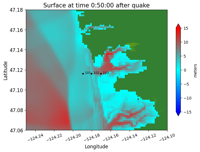
6” resolution#

1” resolution#

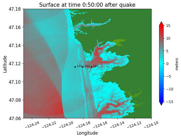
1/3” resolution#

Gauge comparisons#

The plots below were created by the Python script compare_gauges.py. It reads the gauge results for a gauge from each of the 4 _output directories and plots the time series together on the same plot.

Time series at two different gauges are shown: Gauge 101 is just offshore, initially in about 5 meters depth, and Gauge 102 is onshore, at a point that is initially dry.

Note that we plot different quantities at the gauges: at the offshore Gauge 101 it is best to look at the water surface elevation (relative to the vertical datum of the topofile used in this region), while at the onshore Gauge 102 it is better to look at the water depth above the topography.

See Gauge plots for example1 for discussion of why this choice is best, and several other types of plots that you might want to produce at gauges.

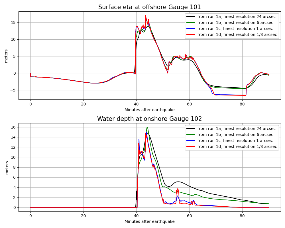
Note from these gauge plots:

Even the very coarse and badly under-resolved simulation of case 1a produces reasonable estimates of the maximum wave height eta offshore at Gauge 101 and also the maximum inundation depth h at the onshore Gauge 102.
Adding more levels of refinement improves the resolution of the results significantly from case 1a to 1b to 1c, but there is little difference between the case 1c results with 1 arcsec resolution and case 1d with 1/3 arcsec resolution. This is a good indication that the results are converging to the “correct” solution for this particular model (solving the shallow water equations with the given topo and dtopo files).

Videos#

Full domain from 3-level run#

Computed using setrun1a.py with 24” resolution around Copalis

The other versions add refinement levels only near Copalis Beach, and so the full domain plots look nearly identical and are not shown below.