Plot the AMR solution along a transect

This Jupyter notebook is available in $GTT/CopalisBeach/exercise1/plot_transect.ipynb within the GeoClaw Tsunami Tutorial.

This notebook shows how to plot a single time frame of the AMR solution and how to extract a one-dimensional transect of the solution from the AMR structure.

%matplotlib inline

from pylab import *
from clawpack.visclaw import gridtools
from clawpack.pyclaw import Solution
import setplot 

Note

The fort.b files needed for plotting the 2D results below are not currently included in the sample_results/_output directory, due to their size (74M). So this notebook only works if you run the code locally and use outdir = _output, or run the fetch_big_sample_results.py script. Choose one of these options in the next cell.

if 1:
    # use this to fetch big_sample_results from the online data repository:
    import os
    if not os.path.isdir('big_sample_results'):
        import fetch_big_sample_results  # fetches directory
    outdir = 'big_sample_results/_output'
else:
    # use this if you have run the code locally to create '_output'
    outdir = '_output'

GTT path is  /home/runner/work/geoclaw_tsunami_tutorial/geoclaw_tsunami_tutorial/GTT
setting GTT =  /home/runner/work/geoclaw_tsunami_tutorial/geoclaw_tsunami_tutorial/GTT
extraction_path =  /home/runner/work/geoclaw_tsunami_tutorial/geoclaw_tsunami_tutorial/GTT/CopalisBeach/exercise1
new_file_fullpath =  /home/runner/work/geoclaw_tsunami_tutorial/geoclaw_tsunami_tutorial/GTT/CopalisBeach/exercise1/big_sample_results

Extracted /home/runner/work/geoclaw_tsunami_tutorial/geoclaw_tsunami_tutorial/GTT/CopalisBeach/exercise1/big_sample_results

Data is cached at:  /tmp/tmpdpkyn7v5/clawpack/geoclaw/GTT_data/CopalisBeach/exercise1/big_sample_results.zip
Directory now exists:  /home/runner/work/geoclaw_tsunami_tutorial/geoclaw_tsunami_tutorial/GTT/CopalisBeach/exercise1/big_sample_results

Use setplot.py to specify how to plot a time frame as a 2D plot

plotdata = setplot.setplot()
plotdata.outdir = outdir
plotdata.print_fignos = [1] # which figno to show
plotdata.printfigs = False  # do not make png file, show here

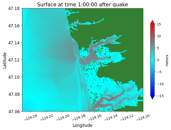
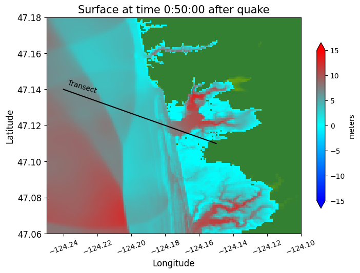
plot a single frame:

plotdata.plotframe(frameno=6)

    Reading  Frame 6 at t = 3600  from outdir = /home/runner/work/geoclaw_tsunami_tutorial/geoclaw_tsunami_tutorial/GTT/CopalisBeach/exercise1/big_sample_results/_output

Define a 1-dimensional transect

x1 = -124.24;  y1 = 47.14
x2 = -124.15; y2 = 47.11
npts = 1000
xtrans = linspace(x1,x2,npts)
ytrans = linspace(y1,y2,npts)

A function to plot one frame together with solution on a transect

The function clawpack.visclaw.gridtools.grid_output_2d can be used to extract values along a one-dimensional transect from a 2D AMR solution. First we read in the full AMR structure and solution using clawpack.pyclaw.Solution

def make_plots(frameno):

    # read in the AMR solution for this time frame:
    framesoln = Solution(frameno, path=outdir, file_format='binary')

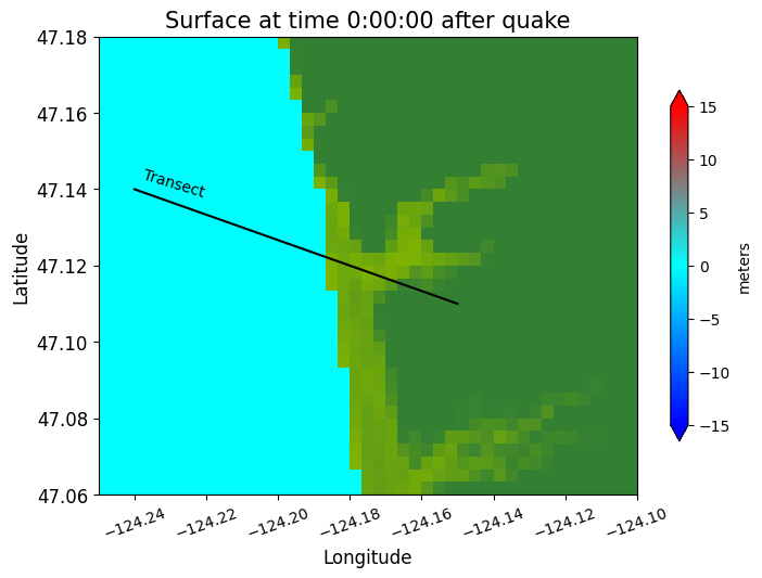
    # Plot the 2D solution:
    plotdata.plotframe(frameno)
    
    # add a line showing the transect location:
    plot(xtrans, ytrans, 'k')
    text(x1+0.002, y1-0.002, 'Transect', rotation=-17)
    
    for method in ['linear', 'nearest']:
        # extract solution along the transect (at discrete points xtrans,ytrans):
        h_trans = gridtools.grid_output_2d(framesoln, 0, xtrans, ytrans, method=method)
        eta_trans = gridtools.grid_output_2d(framesoln, -1, xtrans, ytrans, method=method)
        B_trans = eta_trans - h_trans  # topo reconstructed from eta - h
        
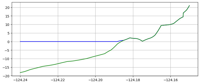
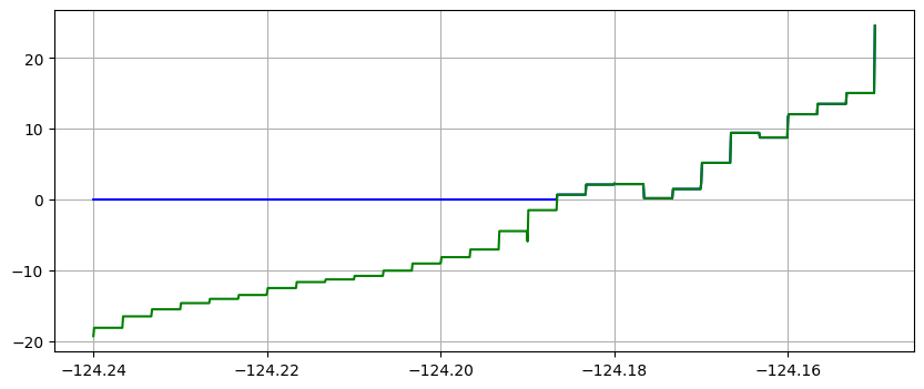
        figure(figsize=(10,4))
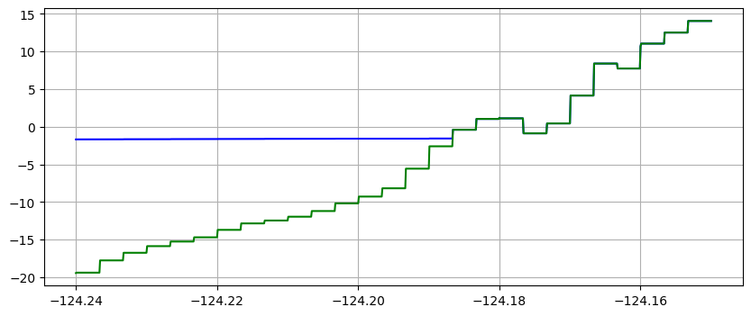
        plot(xtrans,eta_trans,'b')  # plot water surface blue
        plot(xtrans,B_trans,'g')    # plot topo green (on top of eta where h=0)
        ticklabel_format(useOffset=False)
        grid(True)

Apply the function at several times

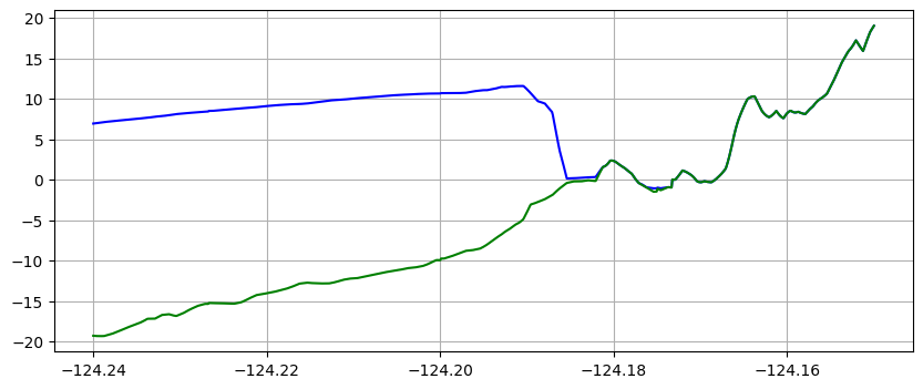
Note in the plots below that the same transect data is plotted in two ways:

1. using piecewise bilinear interpolation between finite volume solution values on the various grids

2. with zero-order interpolation, i.e. the value at each of the points on the transect is simply the value in the finite volume grid cell in which the point lies.

The first method is often preferable since it give smoother looking results, but the second approach better shows the underlying grid resolution of the simulation.

It also shows that at later times the computational grid is more refined than at early times (since the adaptive mesh refinement adds more levels after the tsunami arrives).

make_plots(frameno=0)

    Reading  Frame 0 at t = 0  from outdir = /home/runner/work/geoclaw_tsunami_tutorial/geoclaw_tsunami_tutorial/GTT/CopalisBeach/exercise1/big_sample_results/_output

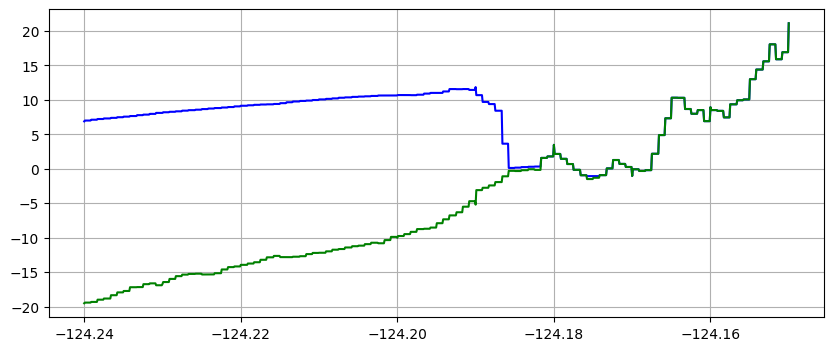
make_plots(frameno=1)

    Reading  Frame 1 at t = 600  from outdir = /home/runner/work/geoclaw_tsunami_tutorial/geoclaw_tsunami_tutorial/GTT/CopalisBeach/exercise1/big_sample_results/_output

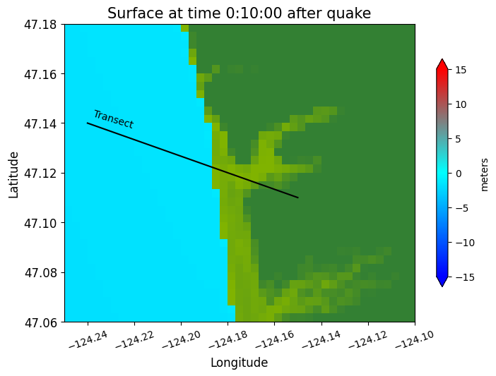
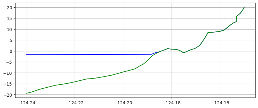
Note in the plots above that the water surface is still at time 10 minutes, but the co-seismic subsidence has dropped both the land and water relative to time 0.

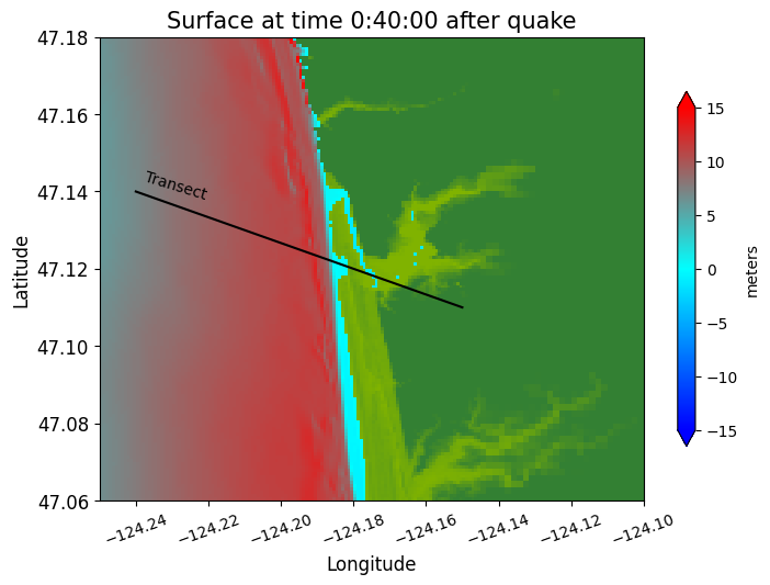
Jumping ahead to 40 minutes, we see the main tsunami arriving:

make_plots(frameno=4)

    Reading  Frame 4 at t = 2400  from outdir = /home/runner/work/geoclaw_tsunami_tutorial/geoclaw_tsunami_tutorial/GTT/CopalisBeach/exercise1/big_sample_results/_output

make_plots(frameno=5)

    Reading  Frame 5 at t = 3000  from outdir = /home/runner/work/geoclaw_tsunami_tutorial/geoclaw_tsunami_tutorial/GTT/CopalisBeach/exercise1/big_sample_results/_output

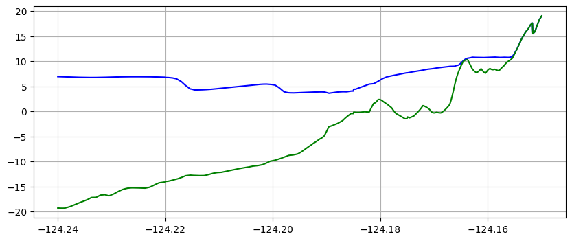
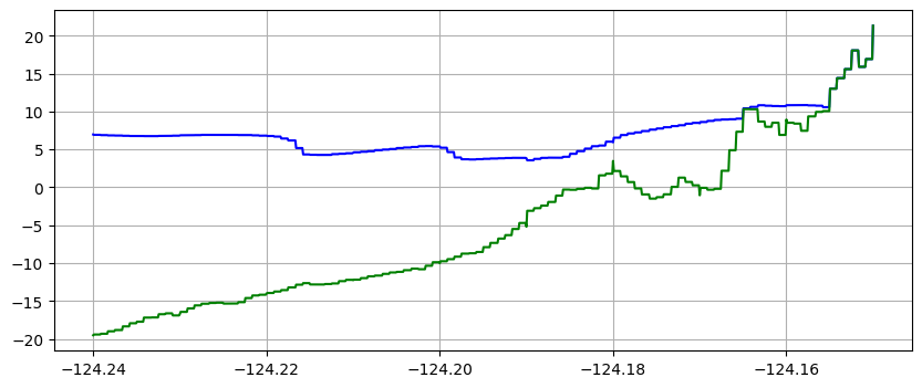
Note that the piecewise constant solution seems to show unequal cell sizes and the topography appears to have some very narrow spikes that do not show up in the linear version. That is because the transect chosen is at an angle to the grid and cuts through the middle of some cells but only nicks a corner of other cells. Since 1000 points are used along the transect, it has much higher resolution than the underlying computational cells, and so there may be one or transect points in a cell even if the transect barely touches it. Bilinear interpolation between the 4 neighboring cell centers gives a much smoother interpolant.