Make topofiles for Copalis Beach (aligned)

This Jupyter notebook is available in $GTT/CopalisBeach/example3/CopalisTopoAligned.ipynb within the GeoClaw Tsunami Tutorial.

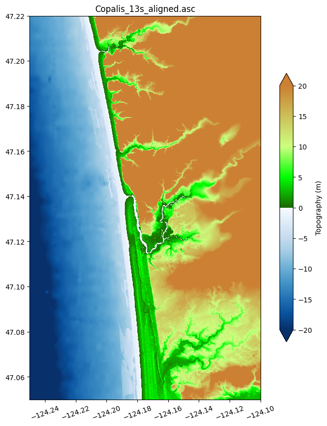
It creates the file Copalis_13s_aligned.asc, which can be used as a topofile in GeoClaw. The resolution is 1/3 arcsecond, and is created by coarsening a DEM with a 1/9” resolution.

Note

A simplified version of this notebook is in $GTT/topo/CopalisTopo.ipynb, where the 1/9” tile is coarsened in the process of downloading (see Make topofiles for Copalis Beach).

The version in this notebook insures that we select the proper subset of the data points to be aligned with cell centers of our computational grid at the 1/3” level, as needed for $GTT/CopalisBeach/example3, where this topofile is also used as the basis for an fgmax grid. See Copalis Beach example3.

The original DEM comes from the NOAA Centers for Environmental Information (NCEI) Continuously Updated Digital Elevation Model (CUDEM) - 1/9 Arc-Second Resolution Bathymetric-Topographic Tiles.

%matplotlib inline

from pylab import *
from clawpack.geoclaw import topotools, kmltools
from IPython.display import Image

Note

See the simplified version of this notebook at Make topofiles for Copalis Beach for more information about the region it covers and the shift used to adjust from NAVD88 to MHW.

Download a subset of 1/9” data and then coarsen:

We will download a subset of this patch data at 1/9” and then coarsen it by 3 so it is at 1/3” resolution, sufficient for our present modeling needs.

Note: The topotools.read_netcdf function has an optional argument coarsen that allows subsampling the data before downloading, to return only every 3rd point in each direction. Calling this with coarsen=3 would result in downloading a smaller file. However, for our purposes in $CHT/CopalisBeach/example3, we want to be careful about which point we use to start subsampling, as explained further below.

#path = 'ncei19_n47x25_w0124x25_2018v1.nc'   # if you downloaded the entire file from webpage
path = 'https://www.ngdc.noaa.gov/thredds/dodsC/tiles/tiled_19as/ncei19_n47x25_w0124x25_2018v1.nc'

extent = [-124.25, -124.1, 47.05, 47.22]

try:
    topo19s = topotools.read_netcdf(path, extent=extent)
    print('Downloaded cropped/coarsened topo \nwith shape: ', topo19s.Z.shape)
except:
    raise Exception('*** failed to read topo data')

Downloaded cropped/coarsened topo 
with shape:  (5508, 4860)

Note that each 1/9” tile has roughly \(9*3600*0.25 = 8100\) points in \(x\) and in \(y\), but this cropped subset is smaller.

Coarsening to 1/3”

In $CHT/CopalisBeach/example3 we will specify an fgmax grid using point_style=4, which means that we will provide a variant of the topofile created here that does not contain the topography, but instead has 0/1 values indicating which points from the file should be used as fgmax points. For this to be useful, we need to make sure that the topo DEM points in our 1/3” topofile exactly agree with the computational points at the finest 1/3” level (i.e. the centers of these finite volume cells).

This means that we want the topo points to be integer multiples of 1/3” (dx13s = 1/(3*3600) degrees) away from the first cell center if we were to have a 1/3” grid starting at the lower left corner of the computational domain we plan to use. This cell center is 0.5 * dx13s away from the domain corner, since we specify the edges of the domain in setrun.py, not the cell center positions.

In the x-direction, here is how many 1/3” cells the first few topo points in topo19s lies from the first cell center location in the bottom left corner:

domain_x_lower = -128.5
dx13s = 1/(3*3600)
first_x_center = domain_x_lower + 0.5*dx13s
(topo19s.x[:6] - first_x_center) / (0.5*dx13s)

array([91799.33301385, 91799.99968059, 91800.66634734, 91801.33301408,
       91801.99968083, 91802.66634757])

Note that (up to rounding error) every third point is an integer multiple away. So we could start sampling at index i1 = 1 (the second point listed above with Python indexing).

i1 = 1

We can do the same calculation in the y-direction:

domain_y_lower = 45.
dy13s = 1/(3*3600)
first_y_center = domain_y_lower + 0.5*dy13s
(topo19s.y[:6] - first_y_center) / (0.5*dy13s)

array([44279.33314166, 44279.9998084 , 44280.66647515, 44281.33314189,
       44281.99980864, 44282.66647538])

From this we see that we can also start with the j1 = 1 index in y.

j1 =1

In order to subsample, remember that in a topofile the indices are in the order (latitude,longitude):

print(f'topo19s.x has shape {topo19s.x.shape}, topo19s.y has shape {topo19s.y.shape}')
print(f'topo19s.Z has shape {topo19s.Z.shape}')
print(f'Note that topo19s.Z[j,i] corresponds to point (x[i],y[j])')

topo19s.x has shape (4860,), topo19s.y has shape (5508,)
topo19s.Z has shape (5508, 4860)
Note that topo19s.Z[j,i] corresponds to point (x[i],y[j])

Subsample by 3 in each direction to go from 1/9” to 1/3”:

x_13s = topo19s.x[i1::3]
y_13s = topo19s.y[j1::3]
Z_13s = topo19s.Z[j1::3, i1::3]

print(f'x_13s has shape {x_13s.shape}, y_13s has shape {y_13s.shape}')
print(f'Z_13s has shape {Z_13s.shape}')

x_13s has shape (1620,), y_13s has shape (1836,)
Z_13s has shape (1836, 1620)

Create a topotools.Topography object with this data

We create a new object and then use the set_xyZ function to set the object’s x,y,Z attributes. Note that this is the proper way to do it rather than just setting e.g. topo13s.x = x_13s, in order for topo13s.X to also be automatically set to the 2D version (with X[j,i] = x[i] and similarly Y[j,i] = y[j]).

topo13s = topotools.Topography()
topo13s.set_xyZ(x_13s, y_13s, Z_13s)

print(f'topo13s.X and topo13s.Y are now also set with shape {topo13s.X.shape}') 

topo13s.X and topo13s.Y are now also set with shape (1836, 1620)

Shift the Z array so that it gives elevations relative to MHW:

Zmhw = topo13s.Z - 2.091
topo13s.set_xyZ(topo13s.x, topo13s.y, Zmhw)

figure(figsize=(10,10))
ax = axes()
topo13s.plot(axes=ax, limits=(-20,20), cb_kwargs={'shrink':0.7, 'extend':'both'})
title('Copalis_13s_aligned.asc')
fname = 'Copalis_13s_aligned.png'
savefig(fname, bbox_inches='tight');
print('Created ',fname)

Created  Copalis_13s_aligned.png

Save this file in .asc format (see Topography data documentation) with 3 digits (mm resolution):

fname = 'Copalis_13s_aligned.asc'
topo13s.write(fname, topo_type=3, header_style='asc', Z_format='%.3f')
print('Created ',fname)

Created  Copalis_13s_aligned.asc

This file can be read into GeoClaw as one of our topofiles.

Create a kmz file to view the topography on Google Earth

The plot above shows the topography file but to see how well it agrees with reality, it is nice to create plots on top of satellite imagery. One nice way to do this is to wrap the plot together with a kml file that positions it on Google Earth into a kmz file:

kmltools.topo2kmz(topo13s, zlim=(-20,20), name='Copalis_13s_aligned')

Will put png and kml files in kmlfiles_Copalis_13s_aligned
Using kml_dpi = 245,figure size 13.224490 by 14.987755 inches
Figure has 1620 by 1836 grid cells of uniform color
Dots per cell in x: 2.000000,  in y: 2.000000
       These should be integers

Created  kmlfiles_Copalis_13s_aligned/Copalis_13s_aligned_land.png
Using kml_dpi = 245,figure size 13.224490 by 14.987755 inches
Figure has 1620 by 1836 grid cells of uniform color
Dots per cell in x: 2.000000,  in y: 2.000000
       These should be integers

Created  kmlfiles_Copalis_13s_aligned/Copalis_13s_aligned_water.png
Extent:   -124.250000  -124.100000   47.050000   47.220000
Created  kmlfiles_Copalis_13s_aligned/Copalis_13s_aligned_topo.kml
kmz file will include:
    Copalis_13s_aligned_topo.kml
    colorbar.png
    Copalis_13s_aligned_land.png
    Copalis_13s_aligned_water.png
Created /home/runner/work/geoclaw_tsunami_tutorial/geoclaw_tsunami_tutorial/GTT/CopalisBeach/example3/kmlfiles_Copalis_13s_aligned/topo_Copalis_13s_aligned_topo.kmz

Opening the resulting kmz file in Google Earth displays the topography plots.

This looks nearly identical to the topofile created Make topofiles for Copalis Beach, but if you zoom in you will see that there are some minor differences since we selected points that are offset by 1/9” from those used in that simplified version.