Make topofiles for Copalis Beach

This Jupyter notebook is available in $GTT/topo/CopalisTopo.ipynb within the GeoClaw Tsunami Tutorial.

It creates the file $GTT/topo/topofiles/Copalis_13s.asc, which can be used as a topofile in GeoClaw. The resolution is 1/3 arcsecond, and is created by coarsening a DEM with a 1/9” resolution.

The original DEM comes from the NOAA Centers for Environmental Information (NCEI) Continuously Updated Digital Elevation Model (CUDEM) - 1/9 Arc-Second Resolution Bathymetric-Topographic Tiles.

Note: This topofile can alternatively be downloaded using the $GTT/topo/fetch_topo1.py script.

%matplotlib inline

from pylab import *
from clawpack.geoclaw import topotools, kmltools
from IPython.display import Image

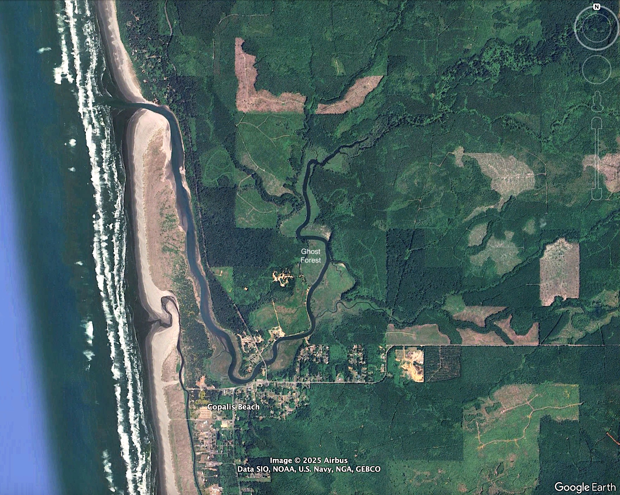
Satellite imagery of the coast around Copalis Beach, WA

(Obtained as a screenshot from Google Earth, and annotated to show the location of the ghost forest.)

Image('images/CopalisTopo0.jpg', width=700)

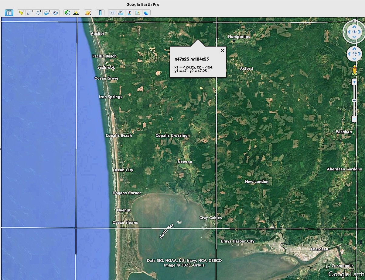
Create a kml file that helps us select the NCEI 1/9” tile to use:

Much of the coast is covered by new DEMs at the 1/9” resolution that each cover 0.25 by 0.25 degrees. The tiles have names like ncei19_n47x25_w0124x25_2018v1.nc where NCEI refers to the National Center for Environmental Information and n47x25_w0124x25 indicates the upper left corner is at (longitude, latitude) \(=(-124.25, 47.25)\).

The Python script make_combined_tiles_kml.py can be used to plot this tiling, which can help you figure out which tile(s) you need to cover the stretch of coastline you are interested in:

run make_combined_tiles_kml

Created  ncei_tile_edges_Cascadia.kml

Open this kml file and click on the tile desired to see its name. You should see something like this…

Image('images/CopalisTile.jpg', width=700)

This tile can be found on the webpage https://www.ngdc.noaa.gov/thredds/catalog/tiles/tiled_19as/catalog.html You can download the entire tile from there, or use the OpenDAP url found at https://www.ngdc.noaa.gov/thredds/dodsC/tiles/tiled_19as/ncei19_n47x25_w0124x25_2018v1.nc.html

#path = 'ncei19_n47x25_w0124x25_2018v1.nc'   # if you downloaded the entire file from webpage
path = 'https://www.ngdc.noaa.gov/thredds/dodsC/tiles/tiled_19as/ncei19_n47x25_w0124x25_2018v1.nc'

Download a subset of this data, coarsened by 3 so it is at 1/3” resolution:

extent = [-124.25, -124.1, 47.05, 47.22]
try:
    topo13s = topotools.read_netcdf(path, extent=extent, coarsen=3)
    print('Downloaded cropped/coarsened topo \nwith shape: ', topo13s.Z.shape)
except:
    raise Exception('*** failed to read topo data')

Downloaded cropped/coarsened topo 
with shape:  (1836, 1620)

Note that each 1/9” tile has roughly \(9*3600*0.25 = 8100\) points in \(x\) and in \(y\), but this coarsened subset is much smaller.

Plot the coarsened subset:

figure(figsize=(10,10))
ax = axes()
topo13s.plot(axes=ax, limits=(-20,20), cb_kwargs={'shrink':0.5, 'extend':'both'});

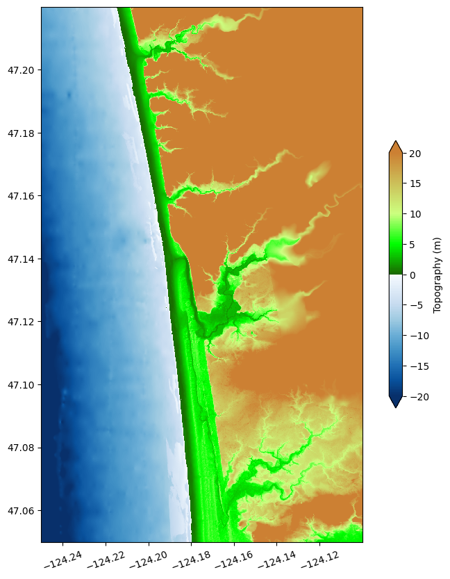
Note that this looks odd since the river mouth seems to be dry.

That’s because this data set is referenced to NAVD88 rather than MHW, which we will use for our tsunami modeling. (NAVD88 is the North American Vertical Datum of 1988, and MHW is Mean High Water, the average water level at high tide.)

The offset can be estimated from the VDATUM website https://vdatum.noaa.gov/vdatumweb/ Choose Region: west coast and Target MHW, then input a latitude, longitude on the Input side and click “Transform” to get an approximate Height…

Image('images/vdatum_copalis.jpg', width=700)

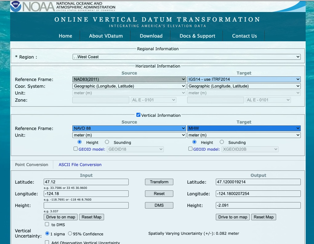
So for Copalis, we should subtract roughly 2.091 m from all the elevations.

(Note: vdatum seems to give approximately 2.1m for all coastal sites on the Cascadia margin, is this correct?)

Shift the Z array so that it gives elevations relative to MHW:

Zmhw = topo13s.Z - 2.091
topo13s.set_xyZ(topo13s.x, topo13s.y, Zmhw)

figure(figsize=(10,10))
ax = axes()
topo13s.plot(axes=ax, limits=(-20,20), cb_kwargs={'shrink':0.7, 'extend':'both'})
title('Copalis_13s.asc')
fname = 'topofiles/Copalis_13s.png'
savefig(fname, bbox_inches='tight');
print('Created ',fname)

Created  topofiles/Copalis_13s.png

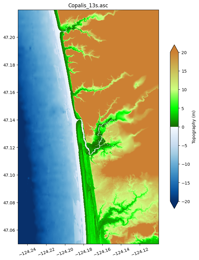
This looks more reasonable.

Save this file in .asc format (see Topography data documentation) with 3 digits (mm resolution):

fname = 'topofiles/Copalis_13s.asc'
topo13s.write(fname, topo_type=3, header_style='asc', Z_format='%.3f')
print('Created ',fname)

Created  topofiles/Copalis_13s.asc

This file can be read into GeoClaw as one of our topofiles.

Create a kmz file to view the topography on Google Earth

The plot above shows the topography file but to see how well it agrees with reality, it is nice to create plots on top of satellite imagery. One nice way to do this is to wrap the plot together with a kml file that positions it on Google Earth into a kmz file:

kmltools.topo2kmz(topo13s, zlim=(-20,20), name='Copalis_13s')

Will put png and kml files in kmlfiles_Copalis_13s
Using kml_dpi = 245,figure size 13.224490 by 14.987755 inches
Figure has 1620 by 1836 grid cells of uniform color
Dots per cell in x: 2.000000,  in y: 2.000000
       These should be integers

Created  kmlfiles_Copalis_13s/Copalis_13s_land.png
Using kml_dpi = 245,figure size 13.224490 by 14.987755 inches
Figure has 1620 by 1836 grid cells of uniform color
Dots per cell in x: 2.000000,  in y: 2.000000
       These should be integers

Created  kmlfiles_Copalis_13s/Copalis_13s_water.png
Extent:   -124.250031  -124.100031   47.049969   47.219969
Created  kmlfiles_Copalis_13s/Copalis_13s_topo.kml
kmz file will include:
    Copalis_13s_topo.kml
    colorbar.png
    Copalis_13s_land.png
    Copalis_13s_water.png
Created /home/runner/work/geoclaw_tsunami_tutorial/geoclaw_tsunami_tutorial/GTT/topo/kmlfiles_Copalis_13s/topo_Copalis_13s_topo.kmz

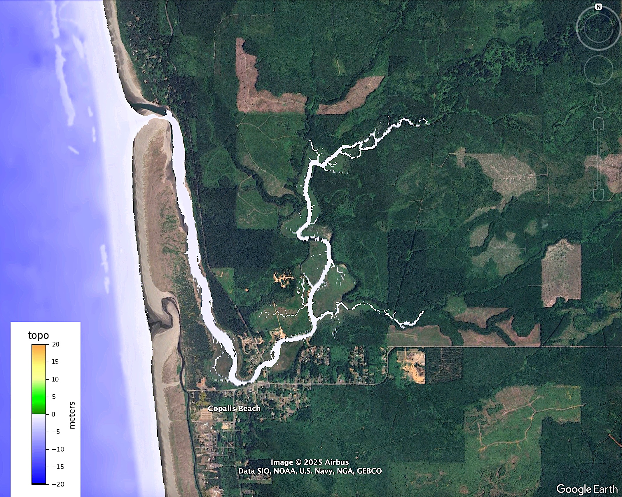
Opening the resulting kmz file in Google Earth displays the topography plots. Here is a screenshot:

Image('images/CopalisTopo1.jpg', width=700)

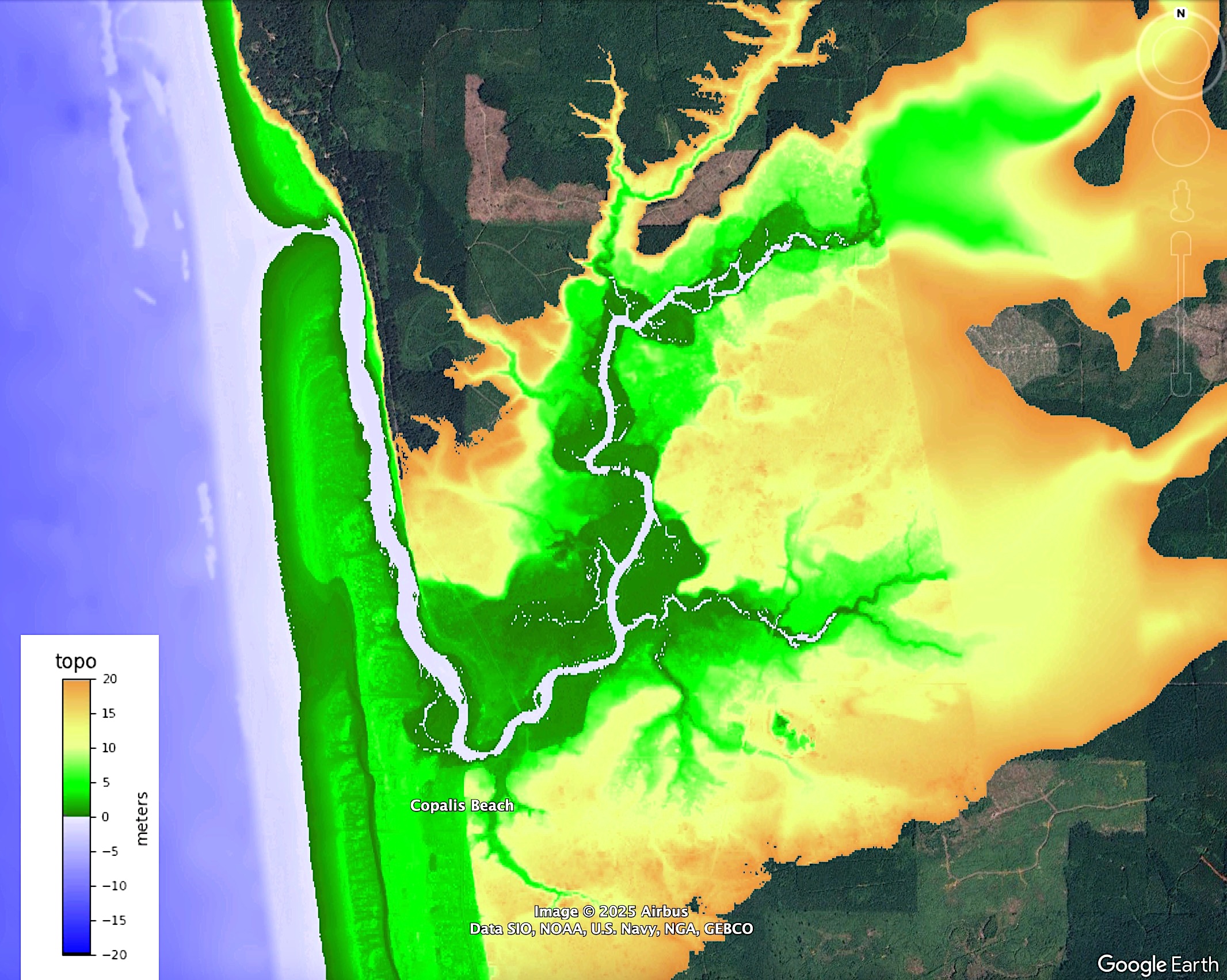
Note that there is an artifact along the east edge, presumably only lower-resolution lidar data was available east of the seam.

If you view the kmz file on Google Earth, you can zoom into to regions of interest. You can also adjust the transparency of the color plot so that the background image show through. You can also turn on or off the land and water layers separately.

If we turn off the land layer and look at only the water layer, which shows the region below B = 0 (which should be roughly MHW), we see the view below. Note from this view that the mouth of the river is slightly farther north in the satelite image than in the DEM.

TODO: Note that the beach is rapidly evolving and perhaps show some historical maps of how much it has changed. Also note that topography in 1700 was very different, and the river probably went straight out to the sea. (So can’t expect to model 1700 event at the ghost forest well on today topography!)

Image('images/CopalisTopo2.jpg', width=700)