The plotting package PyVista makes it easy to produce 3D plots of topography (perhaps overlaid with a water surface).
This is illustrated by two Python scripts in this $GTT/topo directory,
described below.
Simple plot of the Copalis Beach topography
For these examples, we use the topography given by the topofile
$GTT/topo/topofiles/Copalis_13s.asc, which was created using the
Make topofiles for Copalis Beach notebook.
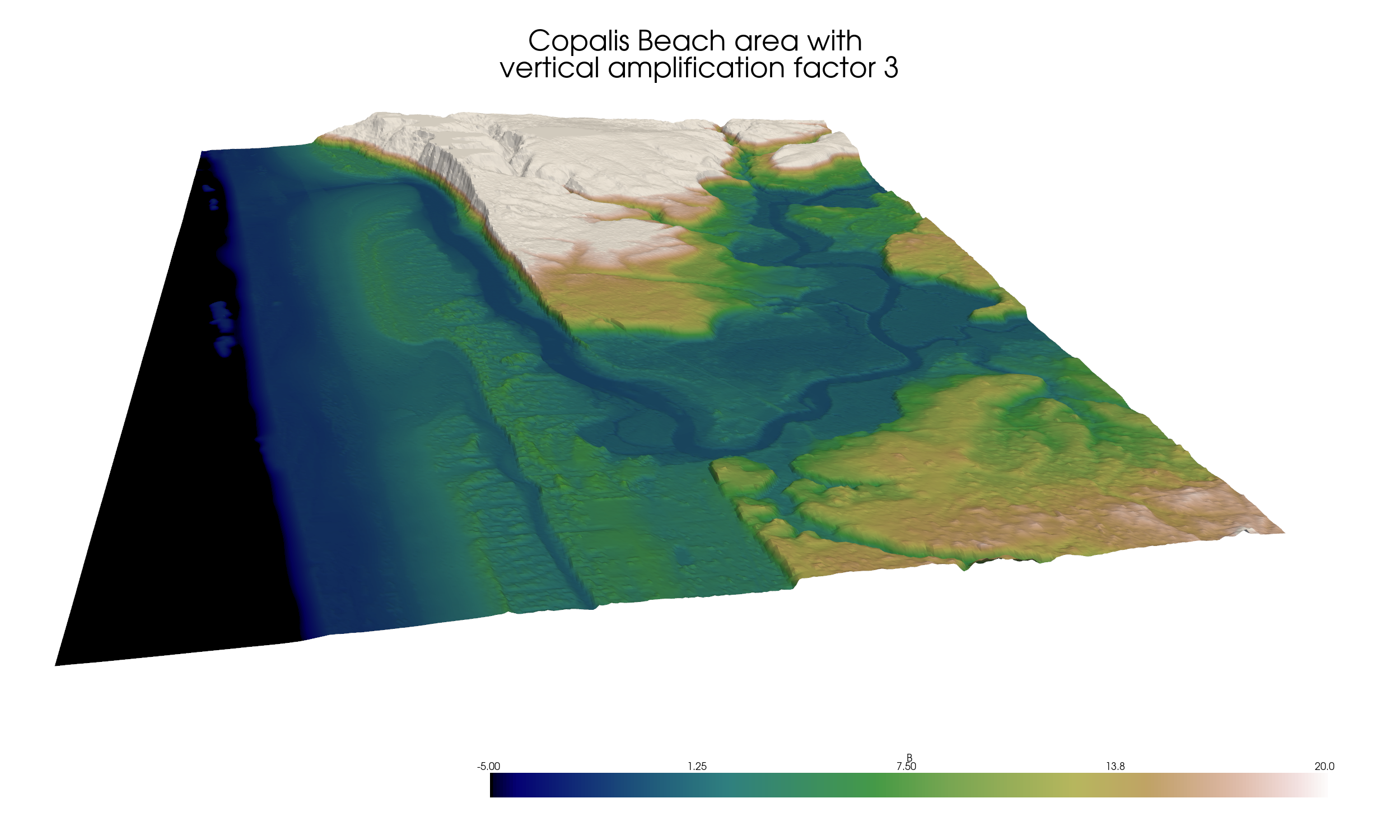
Topography alone
The script $GTT/topo/pyvista_CopalisTopo.py can be used to create a 3D view of
the topography alone. Running the script produces an interactive version where
you can pan, zoom, and rotate (see Interactive 3D plot of topography),
but here we just show a screen shot obtained by setting output = 'png'
in the script:
Topography with the water surface at MHW
Here’s a version in which the water surface at MHW also shown (obtained
by setting show_water = True in the script):
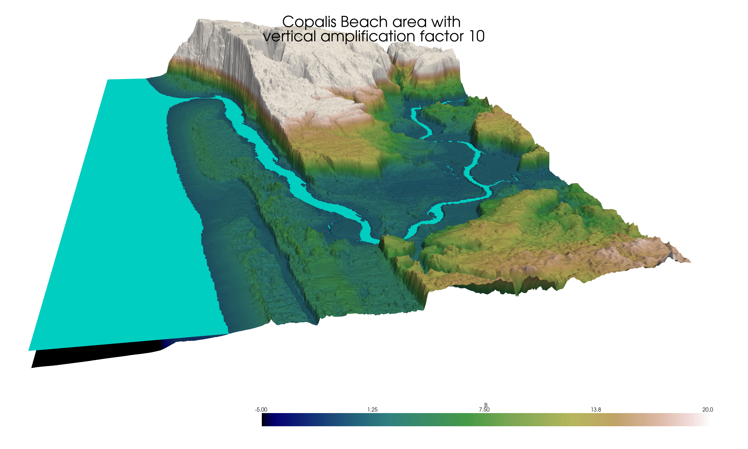
For this figure the vertical exaggeration of topography has also been
increased from 3 to 10 (the warpfactor parameter in the code) to better
show that this is a second surface on top of the topography surface.
Note that vertical exaggeration can help to in visualization but can also
be very misleading if used in excess. In many cases setting warpfactor to
1 or some small value is best.
For an interactive version see Interactive 3D plot of topography. If you have PyVista
installed, then running the pyvista_CopalisTopo.py script will create
a separate window with a similar interactive view.
Changing sea level / coastal subsidence
The more complicated script $GTT/topo/pyvista_CopalisTopo_sealevel.py
can be run to open
an interactive view that allows you to change sea level, in order to explore
what this topography would look like if sea level rises (or following the
co-seismic subsidence of an earthquake).
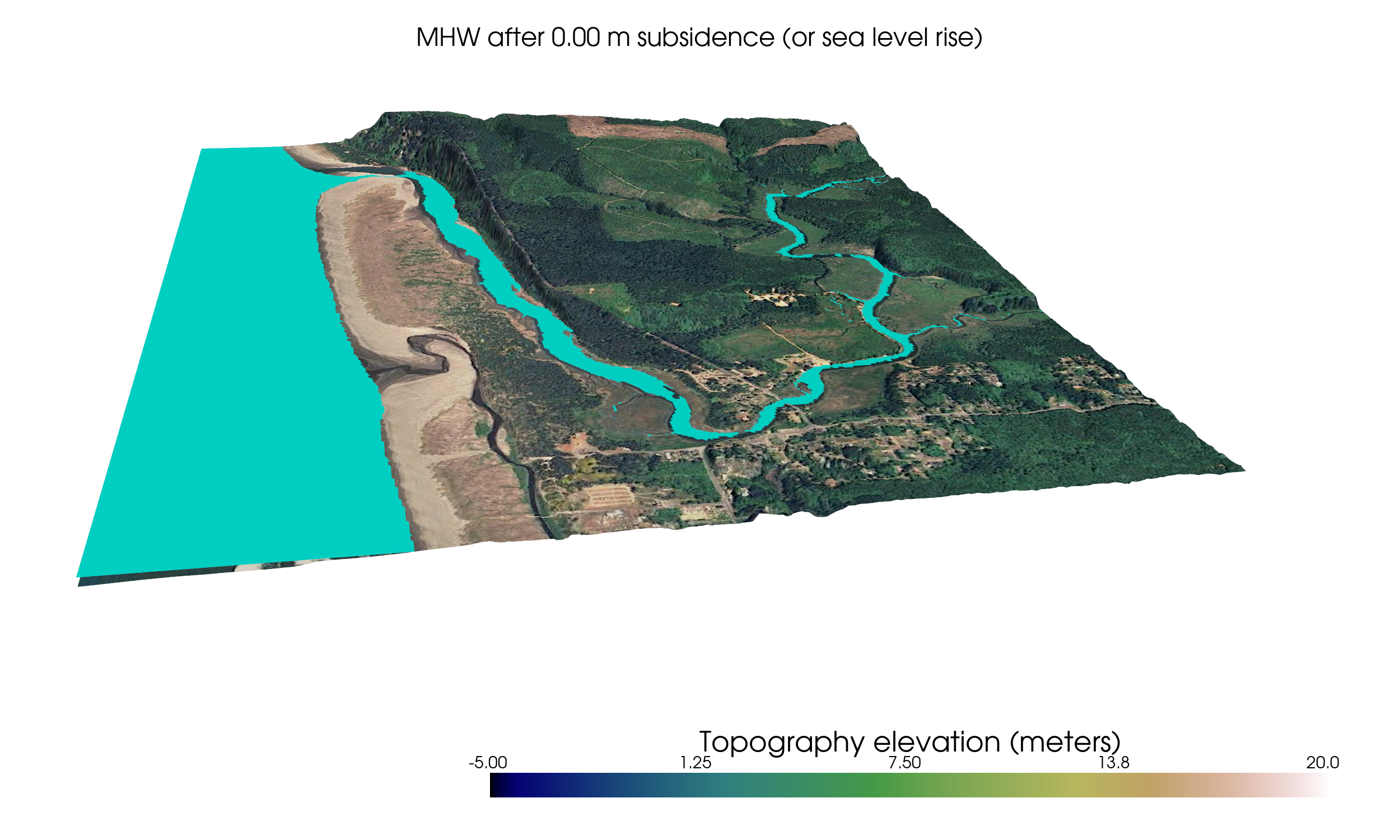
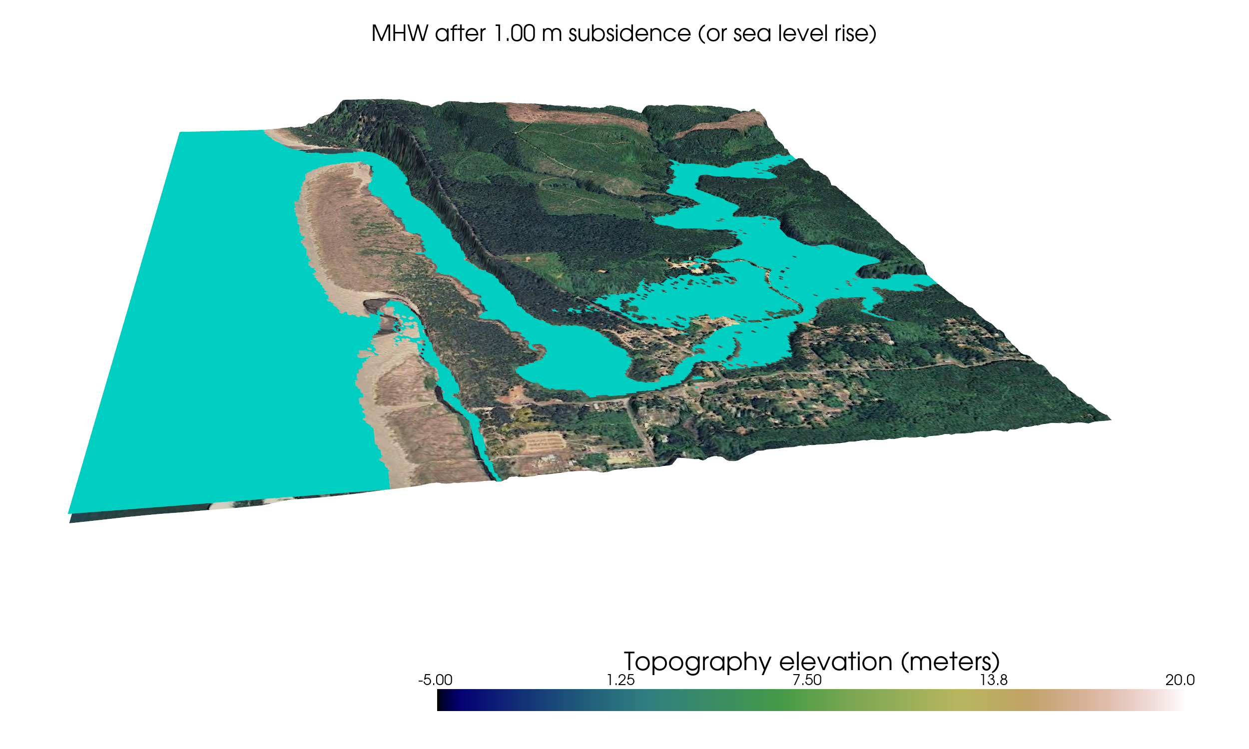
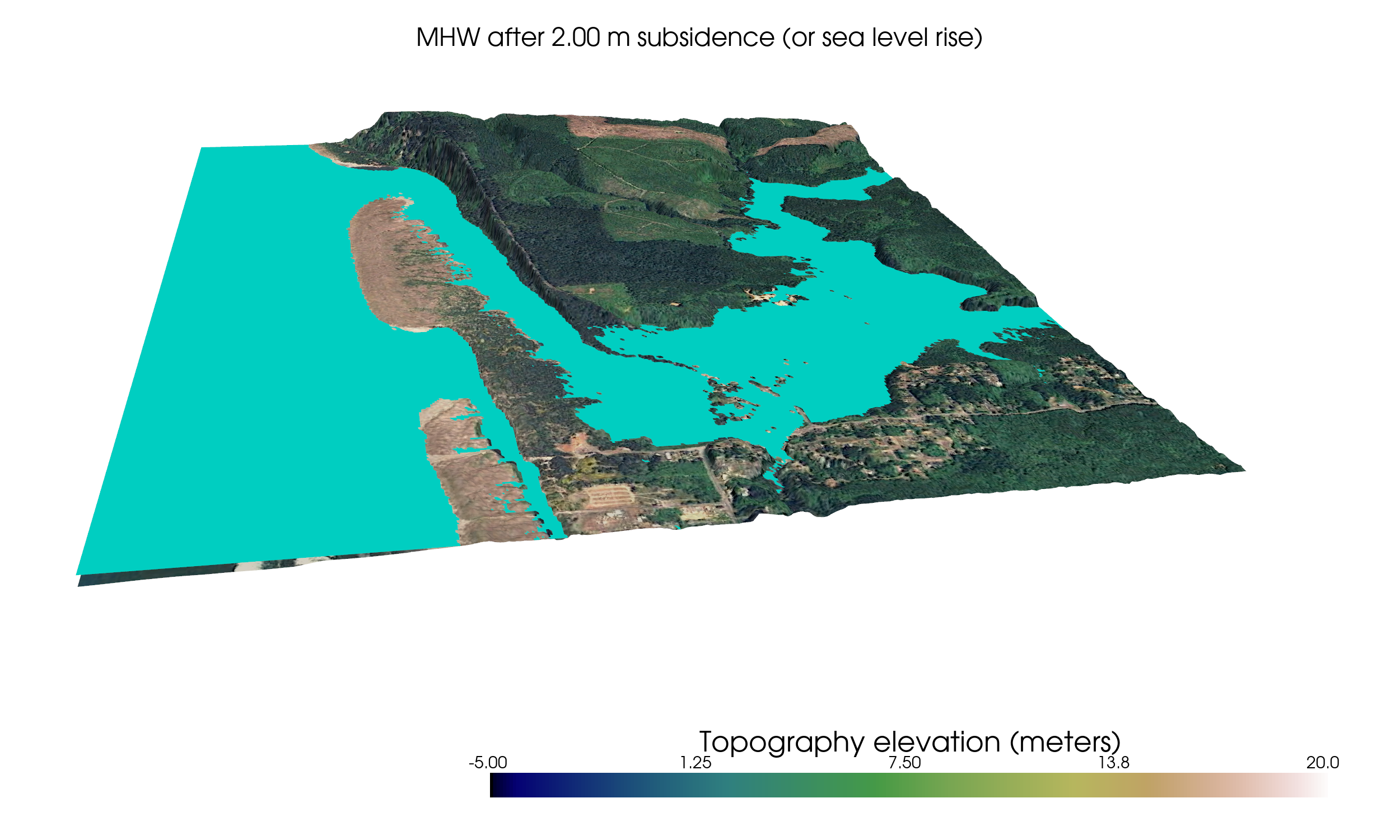
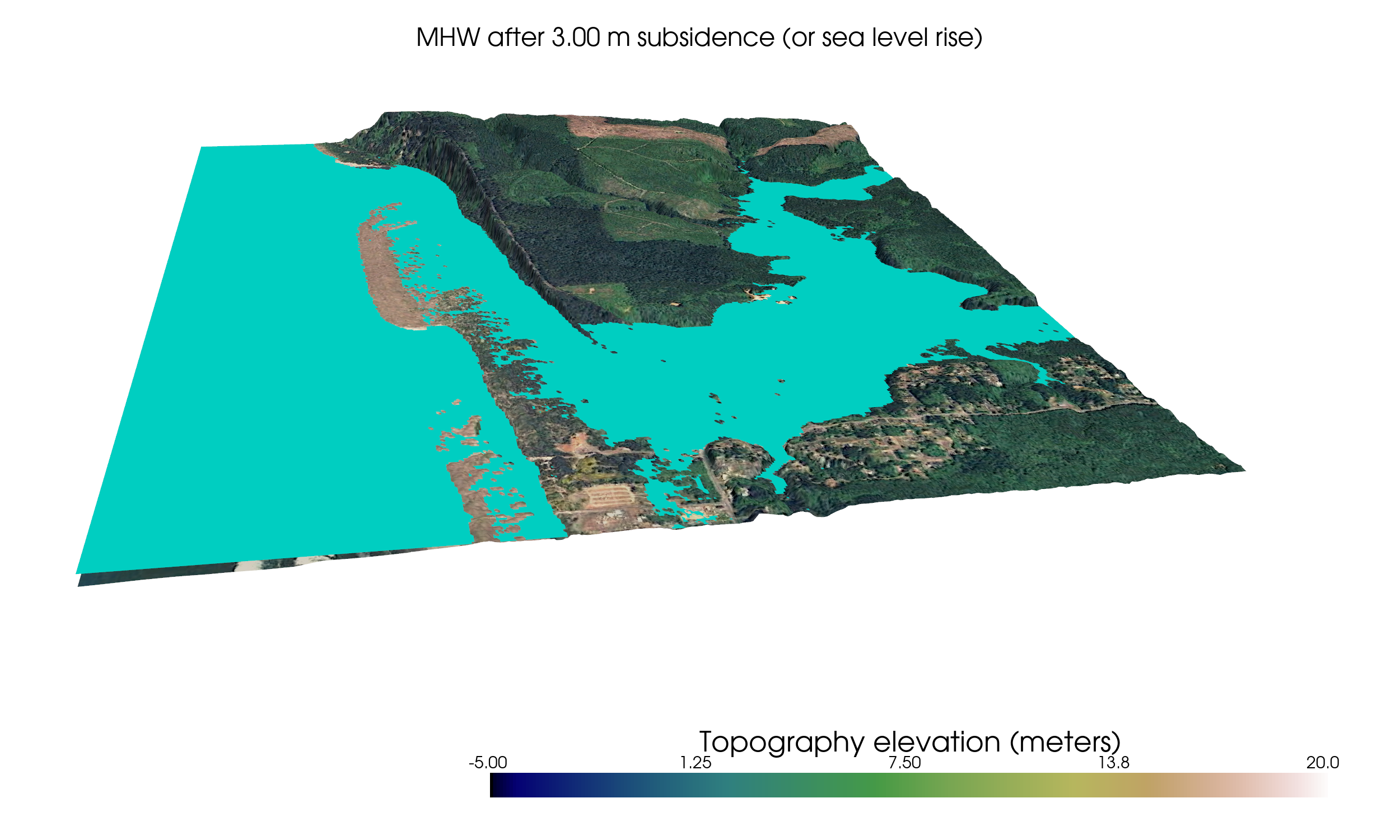
Below are several snapshots for different choices of sea_level
that were produced by setting make_snapshots = True in the script.
The plots below also show that an image can be draped on the topography rather than using a colormap based on elevation. In these figures a screenshot from Google Earth was used as the image, but one could also use a map or other image.
If you run the interactive script, by default there is an unlabelled checkbox in the lower left corner that toggles the image on or off.
The snapshots below show the water surface at four different levels: at MHW and at 1, 2, or 3 meters above MHW.